Scraping Pro-Football-Reference (in R)

Written on February 9th, 2017 by Steven Morse

This post will give a few clean techniques to easily scrape data from Pro-Football-Reference using R. If you are interested in doing NFL analytics but are unfamiliar with R, you might want to check out an introduction like mine over here (or a million others around the web), and then come back here.

Sidenote on language choice: The content of this post is similar to that in this post, and I am posting because I found it was a surprisingly simple process to scrape massive amounts of data from PFR. I was originally going to do this in Python, using the BeautifulSoup package, similar to the nice post here, instead. Veered away from the Python way for other reasons, but I may come back to it in a future post.

Generic scraping function

Let’s write a user-defined scraping function that will scrape one of the nice, clean tables from any one of PFR’s many branches: boxscores, drafts, player data, … we don’t want to have to specify yet.

We’ll use the XML library, which we load into our session with

library(XML)

We’ll make heavy use of the readHTMLTable() function from this library, which takes a character string URL as input and returns a data.frame of the table(s) on that page. (Nice, right?)

Before we write our scraping function, take a look at some typical PFR pages, such as these boxscores from 2011 or 2012. Note the url consists of an unchanging first part, http://www.pro-football-reference.com/years/, followed by the year, and always finishes with a consistent games.htm page name. The pages for the draft, players, etc, all follow a similar pattern.

So let’s write a scraping function like this

scrapeData = function(urlprefix, urlend, startyr, endyr) {
  master = data.frame()
  for (i in startyr:endyr) {
    cat('Loading Year', i, '\n')
    URL = paste(urlprefix, as.character(i), urlend, sep = "")
    table = readHTMLTable(URL, stringsAsFactors=F)[[1]]
    table$Year = i
    master = rbind(table, master)
  }
  return(master)
}

This takes four arguments: that beginning and end of the URL, and the desired start and end year to scrape. Note it stacks each scraped table into a master dataframe, with most recent year ending on top. (You could change this by reversing the order in the rbind() call at the end of the loop.) We also throw in a little cat command to print progress to the console, since this takes a couple seconds per year and we don’t want to get worried.

We are also passing readHTMLTable a stringsAsFactors=F argument, because there is a lot of garbage in these tables that we’ll have to clean out later, and having factors will make it much harder.

Now let’s put it to use on draft data.

Example: Draft data

Let’s load just the drafts from 2010 (just to keep the sample small). With our scrapeData function loaded into the environment, we can just run

drafts = scrapeData('http://www.pro-football-reference.com/years/', '/draft.htm',
                    2010, 2010)

## Loading Year 2010

Let’s take a peek:

head(drafts)

##   Rnd Pick  Tm         Player Pos Age   To AP1 PB St CarAV DrAV   G  Cmp
## 1   1    1 STL   Sam Bradford  QB  22 2016   0  0  5    42   23  78 1773
## 2   1    2 DET  Ndamukong Suh  DT  23 2016   3  4  7    74   59 110     
## 3   1    3 TAM   Gerald McCoy  DT  22 2016   1  5  6    54   54  94     
## 4   1    4 WAS Trent Williams   T  22 2016   0  5  7    57   57  97     
## 5   1    5 KAN     Eric Berry  DB  21 2016   3  5  5    48   48  86     
## 6   1    6 SEA  Russell Okung   T  22 2016   0  1  7    41   36  88     

Looks pretty good. Now let’s make sure it’s cleaned up so we can use it. PFR’s data is remarkably clean, but there’s still some tidying to do.

Cleaning the draft data

If you haven’t noticed, PFR repeats their column headers after every round to make it easier for viewing on a web browser. Unfortunately, this shows up in our table, look:

drafts[30:35,]

##    Rnd Pick  Tm           Player Pos Age   To AP1 PB St CarAV DrAV   G Cmp
## 30   1   30 DET      Jahvid Best  RB  21 2012   0  0  1    13   13  22   0
## 31   1   31 IND     Jerry Hughes  DE  22 2016   0  0  3    30    4 104    
## 32   1   32 NOR Patrick Robinson  DB  23 2016   0  0  1    18   13  81    
## 33 Rnd Pick  Tm           Player Pos Age   To AP1 PB St CarAV DrAV   G Cmp
## 34   2   33 STL   Rodger Saffold   T  22 2016   0  0  5    28   28  83    
## 35   2   34 MIN       Chris Cook  DB  23 2014   0  0  2     8    8  40    

One way to take care of this is to only keep the rows where some column isn’t equal to its own title (any column will do the trick):

drafts = drafts[which(drafts$Rnd != 'Rnd'),]

Next, notice that many of the column names are repeats — TD, Att, Yds, .. — because they refer to Passing, Receiving, Rushing. One way to fix that is to manually adjust the column names like this:

cols = names(drafts)
cols[15] = 'Passing.Att'
cols[16] = 'Passing.Yds'
cols[17] = 'Passing.TD'
cols[18] = 'Passing.Int'
cols[19] = 'Rushing.Att'
cols[20] = 'Rushing.Yds'
cols[21] = 'Rushing.TD'
cols[23] = 'Receiving.Yds'
cols[24] = 'Receiving.TD'
cols[26] = 'Defense.Int'
cols[28] = 'College'
cols[29] = 'link'
names(drafts) = cols

It ain’t pretty but it works. Notice also we gave a name to the unlabeled column that has the link to their College Stats. We’d like to just drop this column as it doesn’t contain any information.

Now the last thing we notice is that everything got scraped as a character string, when many of these columns are numeric. We can use the dplyr package now to quickly mutate a bunch of these columns to numeric. First load in the packages

library(dplyr)

And now we will use the select verb to drop the link column, and the mutate_at verb to convert the desired columns to numbers:

drafts = drafts %>%
  select(-link) %>%
  mutate_at(vars(-Tm, -Player, -Pos, -College, -Year),
            funs(as.numeric(.)))

Now let’s take a last look:

drafts %>% head()

##   Rnd Pick  Tm         Player Pos Age   To AP1 PB St CarAV DrAV   G  Cmp
## 1   1    1 STL   Sam Bradford  QB  22 2016   0  0  5    42   23  78 1773
## 2   1    2 DET  Ndamukong Suh  DT  23 2016   3  4  7    74   59 110   NA
## 3   1    3 TAM   Gerald McCoy  DT  22 2016   1  5  6    54   54  94   NA
## 4   1    4 WAS Trent Williams   T  22 2016   0  5  7    57   57  97   NA
## 5   1    5 KAN     Eric Berry  DB  21 2016   3  5  5    48   48  86   NA
## 6   1    6 SEA  Russell Okung   T  22 2016   0  1  7    41   36  88   NA

Everything is looking good.

A quick plot

Let’s load up ggplot

library(ggplot2)

and we’ll do a quick plot of Career AV vs Pick for offensive skill positions.

(Approximate Value is an attempt to assign a player a number representing his performance for a particular season, developed in-house by Doug Drinen at PFR, and used a lot in analysis of draft value and draft efficiency. Check out the explanation of AV on this blog post on the now-defunct PFR blog.)

I’ll be using a colorblind-friendly palette…

drafts %>%
  filter(!is.na(CarAV), Pos %in% c('QB', 'WR', 'RB', 'TE')) %>%
  ggplot(aes(x=Pick, y=CarAV)) +
  geom_point(aes(color=Pos), size=3) +
  theme_minimal() +
  scale_color_manual(values=c("#E69F00", "#56B4E9", "#009E73", "#F0E442")) +
  geom_smooth(method='lm')

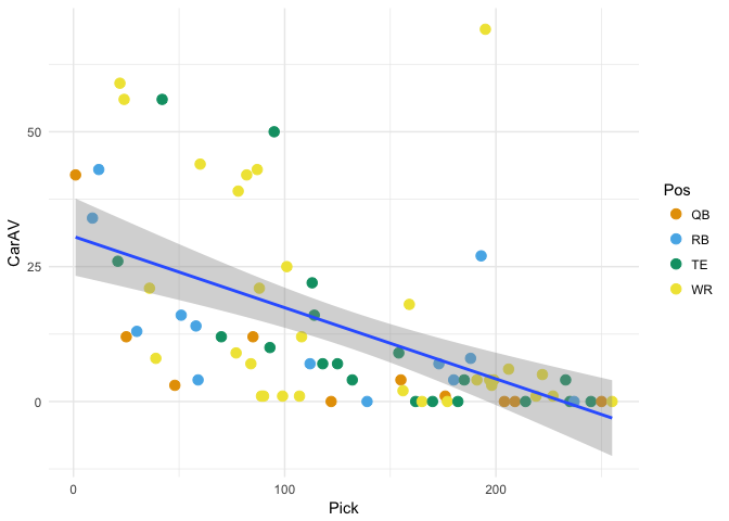
I wouldn’t try to read too much into this, it was mostly just to take a look at the data, but you might argue that WRs outperformed expectations in this draft class! That group of 7 that are way above the trend line are

drafts %>%
  filter(CarAV >= 30, Pos=='WR') %>%
  select(Tm, Rnd, Pick, Player, CarAV)

##    Tm Rnd Pick           Player CarAV
## 1 DEN   1   22 Demaryius Thomas    59
## 2 DAL   1   24       Dez Bryant    56
## 3 SEA   2   60      Golden Tate    44
## 4 CAR   3   78   Brandon LaFell    39
## 5 PIT   3   82 Emmanuel Sanders    42
## 6 DEN   3   87      Eric Decker    43
## 7 PIT   6  195    Antonio Brown    69