Analyzing iMessage conversations

I wanted to do some data science-y analysis of some group conversations I’ve been in for years over iMessage (the Apple ecosystem message app). Questions like: who sends the most texts by hour, most used words, circadian rhythms, maybe some modeling … It turns out that (1) iOS archives all iMessages in a convenient SQL database on your Mac and (2) there is a ton of code out there to read and manipulate this data. So I thought I was in luck.

But I found that these resources tended to neglect group chats (for example this excellent tutorial or many nice Github repos like these PHP scripts). The slick iMessage Analyzer app can handle group chats, and even allows you to export the chat as an easy-to-play-with CSV — but there is a limited menu of queries, it doesn’t differentiate between members of the chat, and it doesn’t make explicit distinction between text vs. attachments.

So in this post I will give some basic recipes for

1. Exporting a group chat as a CSV file, including the sender and type of message (text or attachment).
2. Doing this extraction in a Jupyter/IPython notebook and saving it into a Pandas dataframe
3. Doing some time-series style plots with it. (Might do some text analysis and/or modeling in a later post.)

Checking out chat.db

iOS archives all iMessage chats in a SQL database in /Users/username/Library/Messages/chat.db. (If you poke around in the surrounding folders, you’ll find that each text chain is saved by day in a file you can open in the Message.app application, same with attachments, but this is not helpful for doing anything big.)

We can access this with the built-in SQL tool sqlite3 from the Terminal as

$ sqlite3 /Users/username/Library/Messages/chat.db

(If this gives an “authorization denied” error, try moving a copy of chat.db to a working folder somewhere else, like your desktop, and running sqlite3 from there. The Library folder may be set as non-writeable.)

This brings up a prompt and we can do standard SQL commands — there are lots of references on the web on SQL and sqlite3 help, or you can always try typing .help.

For example, .tables brings up the different tables in the database:

$ sqlite3 /Users/username/Library/Messages/chat.db
SQLite version 3.16.0 2016-11-04 19:09:39
Enter ".help" for usage hints.
sqlite> .tables
_SqliteDatabaseProperties  deleted_messages         
attachment                 handle                   
chat                       message                  
chat_handle_join           message_attachment_join  
chat_message_join

We can also run .schema message to check out the different elements of the message database, or .quit to quit sqlite3.

As an easy example of checking out the database, the handle table is all the IDs and associated phone numbers of people you have messaged. We can check out some of these with a command like:

sqlite> SELECT * FROM handle LIMIT 10;
1|+11231234567|US|iMessage|
...

(Note the semicolon to tell sqlite3 that you’re done with the command! Note also keywords are not case-sensitive, so we can also write select * from handle limit 10;.)

Here’s another simple one to pull messages with a particular contact:

sqlite> SELECT ROWID, text, date FROM message WHERE handle_id=1 LIMIT 10;
4|Hey|503285792
...

We’ll get to how to reformat that “date” number into something useable later.

Exporting a group chat to CSV

Let’s pull an entire group chat history, along with attachment information, and save it to a CSV file. We will use modified commands from this great Github repo.

The following command, entered into a sqlite3 session, will return the entire chat history for chat_id=1:

SELECT ROWID, text, handle_id, 
	   datetime(date + strftime('%s','2001-01-01'), 'unixepoch') as date_utc 
FROM message T1 
INNER JOIN chat_message_join T2 
    ON T2.chat_id=1 
    AND T1.ROWID=T2.message_id 
ORDER BY T1.date;

(We can try to figure out which chat_id we want by running something like SELECT * FROM chat and looking for distinguishing characteristics like the name of the chat.)

This SQL command selects several fields from the message table inner joined with the chat_message_join table. Note we temporarily alias message as T1 and chat_message_join as T2. Also, since all the dates in chat.db are in seconds past January 1, 2001, we convert the date field to a unix_epoch standardized number by adding 01/01/2001 to all the timestamps. We do the inner join using the chat_id and ensuring the ROWIDs and message_ids line up. Finally we order by date.

Now, we can save any SQL query by running the following commands in sqlite3:

sqlite> .mode csv
sqlite> .output test.csv
sqlite> select * from T1;

where our query was SELECT * FROM T1 and it gets saved in test.csv. So we can instead plug in our montrosity from before with the inner join, etc, and save the chat history for chat_id=1 into a CSV file.

Next, to get attachment information, we can use the following command:

SELECT T1.ROWID, T2.mime_type \
FROM message T1 \
INNER JOIN chat_message_join T3 \
    ON T1.ROWID=T3.message_id \
INNER JOIN attachment T2 \
INNER JOIN message_attachment_join T4 \
    ON T2.ROWID=T4.attachment_id \
    WHERE T4.message_id=T1.ROWID \
    AND (T3.chat_id=1)

and follow the same procedure as before to save it into a CSV.

At this point, we can fire up our favorite data analysis tool (Python, R, Excel, whatever) and we have a convenient couple of CSVs saved to play with.

If you’re stopping here, one caveat: the dates are all in Greenwich Mean Time (GMT), so you may want to convert to Eastern standard or something else before you start fiddling around.

Important sidenote: there is probably a slick way to grab the messages and attachments with a single SQL command, and a slick way to do the timezone adjustment in the SQL command …. but I don’t know SQL very well so I’m giving the hacky way that I know works.

Exporting to a Pandas DataFrame

If we’re going straight into an environment like an IPython notebook, we might as well load the query from chat.db directly in our session, instead of saving it as a CSV first.

Fire up a Jupyter/IPython notebook and import the sqlite3, pandas, and datetime packages:

import sqlite3
import pandas as pd
import datetime

(Note sqlite3 is a base package, pandas you may need to install …)

Then we can connect to the database and get a “cursor” to execute commands by running:

conn = sqlite3.connect('/Users/username/Library/Messages/chat.db')
c = conn.cursor()

Let’s say we want chat_id=1.

The following Python commands read in all the messages for a particular chat ID and save it into a Pandas DataFrame by doing an inner join with the message and chat_message_join tables in chat.db. These are the same as before, but just with some backslashes inserted to handle escape characters and newlines:

cmd1 = 'SELECT ROWID, text, handle_id, \
            datetime(date + strftime(\'%s\',\'2001-01-01\'), \'unixepoch\') as date_utc \
            FROM message T1 \
            INNER JOIN chat_message_join T2 \
                ON T2.chat_id=1 \
                AND T1.ROWID=T2.message_id \
            ORDER BY T1.date'
c.execute(cmd1)
df_msg = pd.DataFrame(c.fetchall(), columns=['id', 'text', 'sender', 'time'])

See previous section for a summary of what the SQL commands are doing. In Python world, we execute this command using the cursor in c, retrieve the contents of the command using c.fetchall() and store the result in a Pandas DataFrame. We pick some user-friendly column names that correspond to the fields in SELECT.

Now we want to also load the attachment info for this chat.

cmd2 = 'SELECT T1.ROWID, T2.mime_type \
        FROM message T1 \
        INNER JOIN chat_message_join T3 \
            ON T1.ROWID=T3.message_id \
        INNER JOIN attachment T2 \
        INNER JOIN message_attachment_join T4 \
            ON T2.ROWID=T4.attachment_id \
            WHERE T4.message_id=T1.ROWID \
            AND (T3.chat_id=1)'

c.execute(cmd2)
df_att = pd.DataFrame(c.fetchall(), columns=['id', 'type'])

Same gist as before.

Now we can join the two DataFrames by making the id column the key column and doing a left join:

df = df_msg.set_index('id').join(df_att.set_index('id'))

As noted before, all the time stamps are in GMT (Greenwich mean time). We can translate these to, say, Eastern time by doing

df['time'] = [datetime.datetime.strptime(t, '%Y-%m-%d %H:%M:%S') + datetime.timedelta(hours=-4) for t in df['time']]

which just shifts all the times 4 hours earlier. (This is pretty rough: not all the members of the chat are probably in the same timezone, much less for the duration of the chat, and this doesn’t account for daylight savings.)

Also, the type column is a mix of floats and strings, which is a little annoying, so we’d like it to just be on/off. We can do this with

df['type'] = [1 if type(t) is str else 0 for t in df['type']]

Visualizing the data

Now the fun part. Let’s answer some basic questions about the data dealing only with the time series of the messages and attachments — we’ll save any analysis of the text for a later post. For example: is there more activity on weekends vs. weekdays? how much more active are some members of the chat? how much does activity vary throughout the day? etc.

I’m using an actual group chat for this section, but will keep everything anonymized to protect the innocent (and not so innocent :) ).

Before we start, ensure we import some basic plotting packages:

%matplotlib inline
import matplotlib.pyplot as plt
import seaborn as sns
sns.set_style('white')

The 1st line is just some magic to let you have plots show up inline in the notebook. If you don’t have Seaborn, or don’t like it, you can leave out the last two lines. I’ll also use NumPy for histograms, so you need

import numpy as np

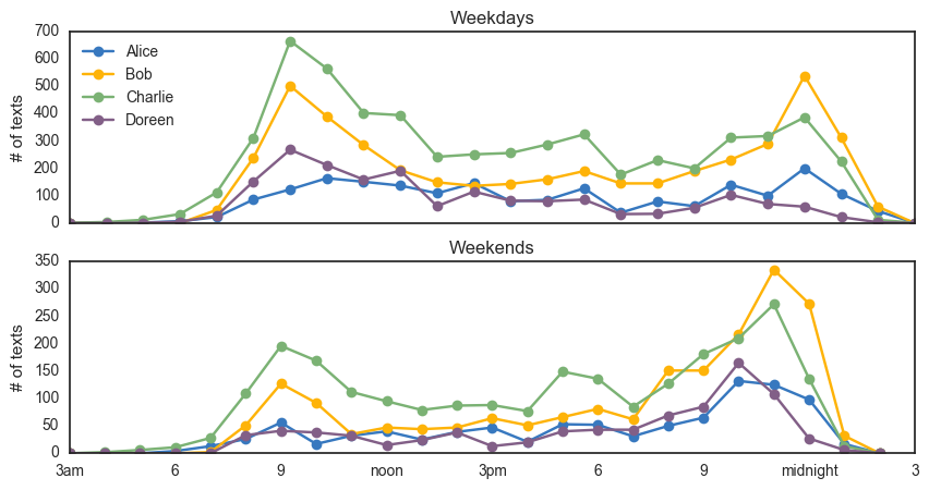
Let’s consider the question: how does activity vary between members, by time of day, and differentiating between weekdays/weekends?

fig, axs = plt.subplots(2,1, sharex=True, figsize=(10,5))
handle_ids, handle_names = [7,34,9,1], ['Alice', 'Bob', 'Charlie', 'Doreen']
colors = ["windows blue", "amber", "faded green", "dusty purple"]
pal = sns.xkcd_palette(colors)
for k,w in enumerate(['Weekdays', 'Weekends']):
    for i,id,name in enumerate(zip(handle_ids, handle_names)):
        if w=='Weekends':
            hours = [d.hour for d in df[df['sender']==id]['time'] if d.weekday() >= 5]
        else:
            hours = [d.hour for d in df[df['sender']==id]['time'] if d.weekday() < 5]
        hist, bins = np.histogram(hours, bins=range(25), density=False)
        axs[k].plot(np.append(bins[3:-1], bins[:3]+24), np.append(hist[3:], hist[:3]), 
                    c=pal[i], linestyle='solid', marker='o', label=name)
    axs[k].set_xticklabels(['3am',6,9,'noon','3pm',6,9,'midnight',3])
    axs[k].set_xticks([3,6,9,12,15,18,21,24,27])
    axs[k].set_ylabel('# of texts')
    if k==0: axs[k].legend(loc=2)
    axs[k].set_title(w)
plt.show()

I’m using a Seaborn color palette using the crowd-sourced xkcd color list. I prefer to do the histogram separately from the plot command (as opposed to plt.hist() for example). The d.weekday() command gives the day-of-the-week for a datetime object, which starts at Monday = 0.

For this group chat, it looks like there are two clear high-activity members (Bob and Charlie) and two not-so-high (Alice and Doreen), and this is consistent on weekdays and weekends. We also see a clear shift from heavier morning activity to heavier evening activity on the weekends.

We now have the tools and data to ask many similar questions: who sends the most attachments (by hour? by members? …), what days of the week are most active, are there lulls or spikes on holidays, etc.

We can also now investigate modeling techniques: how can we capture the obvious circadian rhythms of the above activity plot? how predictive is it? do certain members of the group tend to cause activity from other members or does everyone act independently? Etc. I’m hoping to write about this in a future post, as a toy example for a modeling framework I’ve used in my research called the Hawkes process.