Momentum vs. Acceleration in Gradient Descent

There are some really nice connections between “momentum” and “accelerated” gradient descent methods, and their continuous time analogues, that are well-documented in different pieces throughout the literature, but rarely all in one place and/or in a digestible format. As a result, confusion about these topics crops up in Stack Exchange posts, like here, and there are a handful of blog-style posts aimed at clarification, like here or here or this gorgeous one here.

This is not my research area, but I find this stuff really interesting, and so I want to try to share some of these ideas succinctly in one place in this post in a way I don’t see elsewhere, and also do some experiments.

(By the way, if you also find this a satisfying, accessible topic, and want to bring some of it to (undergraduate) students, here’s an in-class lab I did with my multivariable calculus classrooms last semester.)

Momentum vs. Acceleration

Gradient Descent

Given a function \(f(\mathbf{x})\), a “vanilla” gradient descent (GD) step is

where \(\alpha\) is the stepsize or “learning rate.” In words, we iteratively take small steps in the direction of steepest descent.

With this simple method, we can ensure we are \(\varepsilon\)-close to an optimum in \(O(1/\varepsilon)\) iterations. At face value, this is not great: if you need, for example, 10 iterations for a single digit of accuracy, then you’d need (possibly) 10000 for 4 digits. Two aspects of GD that slow down its convergence are: (1) it moves slowly through long basins where the gradient is small, and (2) it has the tendency to zig-zag, or “hemstitch,” back and forth across ill-conditioned narrow valleys.

Adding momentum

Now consider the modified step below, which I’ll refer to as “classical momentum” (CM), and is typically attributed to Polyak (1964):

Now at each step, we move in the direction of the gradient, but add a little bump if we moved a lot in the previous step, scaled by \(\beta\). Intuitively, this gives our iterates some “momentum,” helps propel us through the long flat basins, and can smooth out some of the zig-zagging.

Under some very specific conditions on \(f(\mathbf{x})\), CM can even guarantee us a speedup to the \(O(1/\varepsilon)\) convergence rate. But we can do even better.

“Accelerating”

Lastly, consider the step below, which I’ll refer to as “accelerated gradient descent” (AGD), and is typically attributed to Nesterov (1983), although good luck finding an online copy of the original paper:

This is nearly the same as CM, but notice that we’re evaluating the gradient away from our current point, based on how much we moved the previous step. Intuitively, this allows the method to incorporate information about the function surface beyond its current position (perhaps we could think of this as approximating second-order information (or curvature)? not sure if this is okay to say).

For example, if we are about to jump over a valley and begin zig-zagging, we will use the gradient near this landing point, which will be facing against our movement, and cancel it out. So we, in a very loose sense, solve the zig-zagging problem. And, because the momentum term is still present, we move quickly through long flat basins.

Nesterov’s AGD only needs \(O(1/\sqrt{\varepsilon})\) to get \(\varepsilon\)-close to the optimum, using the right parameters for \(\alpha\) and \(\beta_k\) and assuming the gradient is Lipschitz continuous. More amazingly, this turns out to be provably as good as we can do given only first order information!

Nesterov’s method

The discussion thus far has been extremely hand-wavy (my preferred mode of discussion). We have only hinted at convergence guarantees, conditions that must hold about the function \(f\), or the parameters \(\alpha\) and \(\beta\) (which actually need to vary with \(k\)) … in fact, we haven’t even stated the methods in the way they are typically written.

Let’s start there. Nesterov’s accelerated gradient descent method, as typically stated (for example here) is

where

and \(\alpha = 1/L\), the reciprocal of the Lipschitz coefficient. (In practice we won’t know \(L\), and so must use the “observed” Lipschitz coefficient up to that point, which would make \(\alpha\) depend on \(k\), but let’s keep \(\alpha\) constant for this short treatment.)

Stated this way, we initialize with a point \(\mathbf{x}_1 = \mathbf{y}_1\) and begin iterating at \(k=1\).

This statement of AGD is (in)famously opaque, and certainly gives no indication why it would give optimal convergence guarantees, although there is recent work to bridge this gap (see this post by Sebastien Bubeck for some references).

The paper by Sutskever et al. shows a way to rewrite Eq. \eqref{eq:nesterov_old} as Eq. \eqref{eq:ag}, which illuminates its connection to classical momentum, or the “heavy ball” method. How do we get there?

Nesterov’s method: re-stated

Again, our goal is to get from AGD as typically stated in Eq. \eqref{eq:nesterov_old} to something more intuitive, like Eq. \eqref{eq:ag}.

Let’s follow the approach in Sutskever et al., who start by reordering the steps of Nesterov’s method so that the \(\mathbf{x}\) and \(\mathbf{y}\) are “off” by one step. (As far as I can tell this is purely superficial.)

Specifically, we start with a point \(\mathbf{x}_{-1} = \mathbf{y}_0\), and begin iterating with \(k=0\). This means Eq. \eqref{eq:nesterov_old} becomes

where now we set \(a_0 = 1\) because it corresponds to the old \(a_1 = (1+\sqrt{1+0})/2=1\).

It is still not at all obvious how Eq. \eqref{eq:nesterov} is equivalent to the one-liner Eq. \eqref{eq:ag}. The supplementary material for the Sutskever paper walks through this, and this post also shows the derivation, but I’ll rehash it briefly here.

First define \(\mathbf{v}_k = \mathbf{x}_k - \mathbf{x}_{k-1}\) and \(\beta_k = \frac{a_k - 1}{a_{k+1}}\). Now the second equation in \eqref{eq:nesterov} can be rewritten

and we can substitute that into the first equation in \eqref{eq:nesterov} to get

Using this to get an expression for \(\mathbf{x}_k\), and substituting into the definition of \(\mathbf{v}_k\), we find

which, altogether, we could write succinctly as

And now we see this can easily be combined into a one-liner (substitute the first into the second and use the fact \(\mathbf{v}_k = \mathbf{x}_k - \mathbf{x}_{k-1}\).)

More importantly, notice we could have also written our momentum one-liner from Eq. \eqref{eq:cm} like this instead:

It is worth comparing Eq. \eqref{eq:nesterov2} and \eqref{eq:momentum2} for a moment, as Sutskever et al. do to begin their paper. This again reveals the difference between CM and AGD comes where we evaluate the gradient. In CM, we evaluate it at our current point. In AGD, we evaluate it at a little nudged distance in the direction of our momentum.

A quick experiment

Using constant stepsizes, we can do a quick experiment to visualize the difference in the methods. Here I’m using the popular Rosenbrock test function (the “banana” function!),

with \(a=1, b=10\). Note this has a global optimum at \((1,1)\). We will compare the methods as stated in Equations \eqref{eq:gd}, \eqref{eq:cm}, and \eqref{eq:ag}.

With constant stepsize \(\alpha=0.015, \beta=0.7\), starting at \((0.4, 0.4)\) and taking exactly 50 steps, we get:

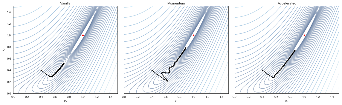
This shows “vanilla” gradient descent exhibiting monotonically decreasing error, but very slow convergence once it reaches the long, flat basin containing the global optimum. Adding momentum causes us to lose the monotonic decrease guarantee, as we are oscillating all over the place, but we are nevertheless able to speed through the flat basin. The shifted gradients used in AGD prevent it from the oscillation in CM, but we maintain the fast convergence.

There is a more thorough experiment on the post I mentioned earlier where he actually shows you can get different results using different formulations of the same essential method.

Continuous time limits

A really beautiful interpretation of momentum and accelerated methods comes as we consider the continuous time limit of the discretized iterations. This is discussed in the literature in many places, like this paper by Su et al., and posts like this nice Distill.pub article. But it doesn’t seem to be part of the canonical first treatment of gradient descent methods, which I think is a shame.

Here’s my version of this story. Consider a particle with mass \(m\) with position \(\mathbf{x}(t)\), being acted on by a (conservative) force field \(\mathbf{F} = -\nabla f(\mathbf{x}(t))\), subject to a frictional force which is proportional to its velocity. By Newton’s law, this gives the second order differential equation

Now, consider a massless particle in this system (\(m=0\)). This simplifies Eq. \eqref{eq:diffeqbase} to the first order differential equation

If we substitute the finite difference approximation

into Eq. \eqref{eq:diffeq_gd} and do a little rearranging, we get

which we recognize as (vanilla) gradient descent. Equivalently, it is an forward Euler method step on Eq. \eqref{eq:diffeq_gd}. Note that the stepsize \(\alpha = \frac{\Delta t}{h}\) gets bigger as we take longer “time” steps, but smaller as we increase the “friction” coefficient in the system.

Now assume \(m>0\), and consider again the original second order differential equation. Apply the approximation from before, and the second order difference approximation

to get (after some careful algebra fiddling)

which is the “momentum” step from Eq. \eqref{eq:cm}.

So if gradient descent approximates the path of a massless particle moving down a hillside, gradient descent with momentum approximates a large heavy ball rolling down hill.

(And in fact, it’s often referred to as Polyak’s “heavy ball method”.)

I believe what Su et al.’s paper does is show that you can use this same framework to get to the AGD scheme, if you select the damping (friction) coefficient exactly correctly at each iteration, but I haven’t worked through this.

Parting thoughts

This post hasn’t touched on the application of these gradient descent modifications to the stochastic setting, i.e. stochastic gradient descent (SGD). My understanding is, although momentum can in general be counterproductive in the final stages of convergence when our gradient is noisy, it can, for example, be extremely useful in the early, transient, or exploratory phase. See: the Sutskever paper, and I’ve also been working through this paper by Mandt et al., and this recent one by Zeyuan Allen-Zhu (who also wrote a paper on AGD as a linear coupling of GD and Mirror Descent, see here).

I hope this post has been interesting and/or useful to you. I’ll end with posting the code for the experiment. Feedback always welcome.

Code for the experiment

I’m working in a Jupyter notebook so my imports are

%matplotlib inline
import matplotlib.pyplot as plt
import numpy as np

First we define the Rosenbrock “banana” function (yes I still think this is funny) and its gradient,

def f(x, a=1, b=100):
    x1, x2 = x[0], x[1]
    return (a-x1)**2 + b*(x2-x1**2)**2

def gf(x, a=1, b=100):
    x1, x2 = x[0], x[1]
    return np.array([
        -2*(a-x1) - 4*b*x1*(x2-x1**2),
        2*b*(x2-x1**2)
    ])

Then we define a multipurpose minimize function a la scipy.optimize. This stops when it reaches maxsteps or the function changes by less than tol,

def minimize(hh, gradh, x0, args={}, method='gd', 
             alpha=0.1, beta=0.1, maxsteps=10, bound=1e3, tol=1e-3):
    if method not in ['gd', 'cm', 'ag']:
        print('Unrecognized method.')
        return None
        
    # store trace of updates
    w = np.zeros((maxsteps,2))
    
    # convenience function references
    def h(x): return hh(x, **args)
    def gh(x): return gradh(x, **args)
    
    # initial step always simple gradient
    w[0] = x0
    w[1] = w[0] - alpha*gh(w[0])

    for k in range(1, maxsteps-1): 
        if method=='gd':
            w[k+1] = w[k] - alpha*gh(w[k])
        elif method=='cm':
            w[k+1] = w[k] - alpha*gh(w[k]) + beta*(w[k] - w[k-1])
        elif method=='ag':
            vk = w[k] - w[k-1]
            w[k+1] = w[k] - alpha*gh(w[k]+beta*vk) + beta*vk
            
        if np.linalg.norm(w[k+1]) > bound:
            print('Unbounded behavior.')
            break
            
        if k % 10 == 0 and np.abs(h(w[k+1]) - h(w[k])) <= tol:
            break
        
    return w[:k+1]

And last but not least, producing the visualization,

fargs = {'a':1, 'b':10}
x0    = [0.4, 0.4]
kws   = {'alpha': 0.015, 'beta': 0.7, 'maxsteps': 50}

x = np.linspace(0, 1.5, 500)
y = np.linspace(0, 1.5, 500)
X, Y = np.meshgrid(x, y)
Z = f([X,Y], a=1, b=10)

fig, ax = plt.subplots(1,3, sharey=True, figsize=(16,5))
for i,(name,m) in enumerate([('Vanilla','gd'), ('Momentum', 'cm'), ('Accelerated', 'ag')]):
    w = minimize(f, gf, x0, args=fargs, method=m, **kws)
    ax[i].contour(X, Y, Z, levels=np.logspace(-1.5,  3.5, 50, base=10), 
                  cmap='Blues_r', alpha=0.4)
    ax[i].scatter([1],[1], c='r', s=20)
    ax[i].plot(w[:,0], w[:,1], 'k.-')
    ax[i].set(xlabel=r'$x_1$', title=name)
ax[0].set(ylabel=r'$x_2$')
plt.tight_layout()
plt.show()