Gambler's walk - some simulations in Python

In the previous post, we covered the basics of how odds connect to bet payouts and probability, and how this changes when a bookmaker is involved taking a cut. In this post, let’s take a look at what kind of dynamics that creates over time. As I mentioned before, I’m writing this mostly as notes-to-self, and please note I’m not a professional gambler so if you’re looking for that kind of experience as context, see you later!

Even-money martingales

So before we looked at how if you bet over and over and the payout was calibrated to the probability, your average winnings would tend to zero. But we also pointed out this was not very useful, since in reality your winnings are not an average, they are cumulative! (If you lost 100 times in a row, your average winnings would be -1, but your total winnings are -100.)

Examining cumulative winnings gets us into the territory of stochastic processes. This subject is a deep ocean but let’s skim over some interesting wave tops.

Let \(B_t\) represent your bankroll, and consider the process defined by \(B_{t+1} = B_t + W_t\) where \(W_t\) is a random variable representing winnings at time \(t\).

In the case of an even-money bet, we have \(W_t=1\) with probability \(p\) and \(W_t=-1\) w.p. \(q=1-p\). Notice that \(\mathbb{E}[W_t] = p + q(-1) = 2p - 1\), so when \(p=1/2\), we have \(\mathbb{E}[W_t]=0\) and therefore \(\mathbb{E}[B_{t+1}] = B_t + \mathbb{E}[W_t] = B_t\). This property makes the even-money bet on 50/50 odds a martingale — it’s expected value at the next step is equal to its current value. (Note: not to be confused with the “martingale” betting strategy, which says to double your money after every loss.)

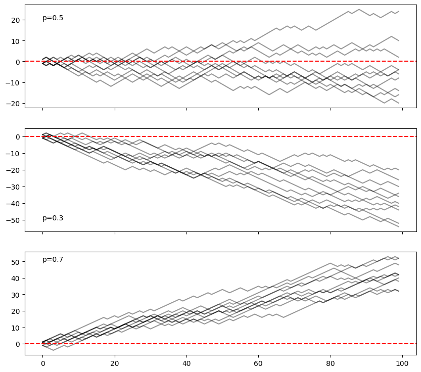
If we keep it an even-money bet, but increase the probability to \(>1/2\), then the bet is in our favor (we should have to pay more for such favorable odds!), our per-bet EV is \(>0\) and our bankroll will exhibit positive drift over time. With even-money bets but \(p<1/2\), the opposite: negative drift. Let’s sanity check this so far with a simulation.

import matplotlib.pyplot as plt
import numpy as np

fig, axs = plt.subplots(3,1, figsize=(10,9), sharex=True)

N = 100     # number of steps
m = 10      # number of sims 
t = np.arange(N)

for i, p in enumerate([0.5, 0.3, 0.7]):
    for _ in range(m):
        # get mask where team wins
        mask = np.random.rand(N) < p

        # compute W_t
        win = np.where(mask, 1, -1)

        # plot B_t + W_t with cumsum
        axs[i].plot(t, np.cumsum(win), 'k-', alpha=0.4)

    # show "ruin" line (0 money)
    axs[i].axhline(y=0, color='r', linestyle='--')

    axs[i].text(0, [20, -50, 50][i], f'p={p:.1f}')

plt.show()

Fortune or Ruin

We notice we pass \(B_t=0\) a lot, which is technically not possible in real life: once your bankroll goes to zero, you are “ruined” and the game stops. We can workout some properties of this event.

Let’s define \(P(i)\) as the probability of reaching some goal bankroll of \(N\), before hitting 0 (“ruin”), given a starting amount of \(i\). With \(p\) and \(q\) again representing the probability of win/loss of 1 unit, we know

We can re-express this as a linear recurrence and deduce (this is straightforward but takes a little work I’m not going into here) the general formula

which for \(p=1/2\) reduces to \(P = b/N\).

And then the probability of reaching ruin before hitting this bankroll is just \(1-P\). (The sequence always ends with us hitting \(N\) or \(0\), so the proportion of times we hit \(N\) is exactly 1 minus the proportion of times hitting 0.)

Let’s test these out in simulation.

np.random.seed(315)

n = 50      # num sims
m = 500     # max steps
p = 0.5

b = 5       # starting bankroll
N = 10      # "winning" bankroll

winners = 0
losers = 0
ratio = []

fig, axs = plt.subplots(2,1, figsize=(10,8))

for k in range(n):
    results = np.random.rand(m)
    mask    = results < p
    win     = np.where(mask, 1, -1)
    walk    = np.append([b], b + np.cumsum(win))

    # find first occurrence of b or N
    end_idx = np.where((walk >= N) | (walk <= 0))[0]
    if len(end_idx) > 0:
        walk = walk[:end_idx[0] + 1]

    axs[0].plot(range(walk.shape[0]), walk, 'k-', alpha=0.5)
    
    e = walk[-1]
    axs[0].scatter(walk.shape[0] - 1, e, c='b' if e==N else 'r')

    if e == N:
        winners += 1
    elif e == 0:
        losers += 1

    ratio.append(winners / (k+1))

axs[0].set_xlabel('Step')
axs[0].set_ylabel('Bankroll')

axs[1].plot(range(n), ratio, 'c-')
axs[1].plot([0,n], [b/N]*2, 'k--')
axs[1].set_xlabel('# Simulations')
axs[1].set_ylabel('Ratio of wins')

plt.show()

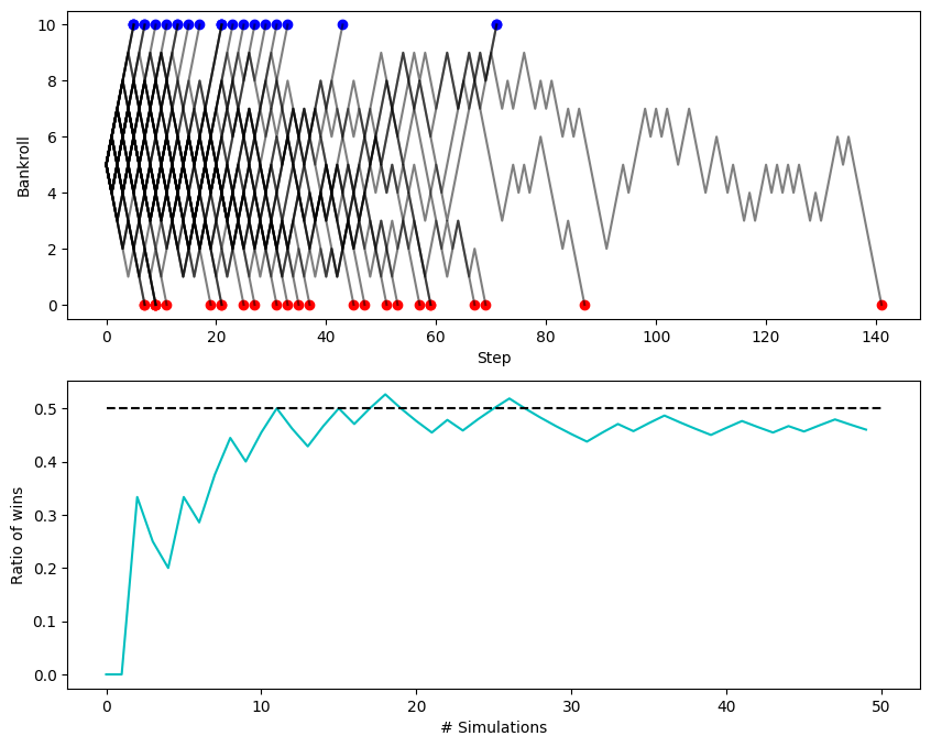
So we see as the number of simulations grow, our ratio of “winning” to “bankrupt” approaches the theoretical mean of \(b/N\) which in this case is 0.5.

If I play 20 hands how likely am I gonna go broke?

The previous section has never been satisfying to me because often you really don’t care whether you will reach your cash-out threshold or not, but how long you have to play, what’s your “broke horizon”. To me there is this sense of, I don’t know what my cash-out point is, but I know I want to play about 20 hands and see where I’m at, so what’s my chances of going broke before I get there?

Another related thought is, if we’re, say, 90\% likely to hit bankruptcy before our winning criteria, but neither condition is going to happen until we’re a million steps in, then maybe we’re less concerned than a more volatile situation where we are guaranteed to hit either riches or ruin within the first 5 bets.

To frame this like before, let’s say what is the “probability of ruin before time \(T\)”, or \(\text{Pr}(\text{ruin by time }T)\). We can actually derive an expression for this in closed form:

which is a little crazy looking. First let’s try to make sense of the formula at face-value, then we’ll do a hand-wavy derivation, then some code to test it in simulation.

First we have a sum over probabilities of hitting ruin at exactly some timing \(k\), which if we sum every possible \(k\), we get the total probability of (any) ruin by time \(T\) (because we’ve got every possible way it could happen added together). Notice we can’t hit 0 before \(b\) steps because our problem setup is that we’re going in \(+1\) and \(-1\) betsizes and starting with \(b\), so the sum starts at \(k=b\).

So let’s think about a single term in this sum, the probability of hitting 0 at exactly \(k\). We want to think about all the possible paths of getting to 0, in exactly \(k\) steps, starting at \(b\). After \(k\) steps, we’ll have \(M\) steps of +1, and \(k-M\) steps of -1, giving \(X_k = b + (+1)M + (-1)(k-M)\). We want \(X_k=0\), giving \(b+2M-k=0\) or \(M=(k-b)/2\). There are \(k\) choose \(M\) ways to choose these \(M\) +1’s, the binomial coefficient term. And out of all these paths, a ratio of \(b/k\) of them will stay above the \(X=0\) axis the whole time, by a symmetry/reflection principle of random walks. And lastly, each of these \(k\) steps is equiprobable, with a chance of \((1/2)^k\).

I’m a little skeptical of this formula, so let’s sanity check in simulation.

from scipy.special import comb   # for binom coefficient

First, let’s check the sum giving probability of ruin by time \(T\). As \(T\) gets bigger (more opportunities to lose) or \(b\) gets smaller (less starting buffer), we should see the probability go up.

fig, ax = plt.subplots(1,1, figsize=(8,6))

Ts = range(4, 10)
colors = plt.cm.Blues(np.linspace(0,1, len(Ts)))

for i, T in enumerate(Ts):
    probs = []
    for b in range(2, T+1):
        probs.append(
            np.sum([(b / k) * comb(k, (k-b)/2, exact=True) * (0.5 ** k) for k in range(b, T+1, 2)])
        )

    ax.plot(range(len(probs)), probs, color=colors[i], marker='o', linestyle='-', label=f'T={T}')

ax.set_ylabel('Pr')
ax.set_xlabel('b')
ax.set_title('Pr(ruin by time T | X0=b)')
ax.legend()
plt.show()

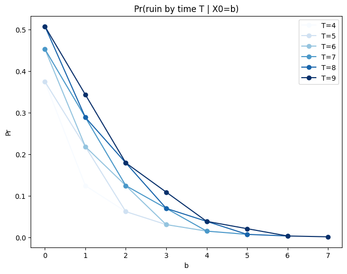
Checks out. Let’s now simulate a bunch of random walks and keep track of how many times we were ruined before some time \(T\), and compare our running average over more and more sims to the theoretical value from the formula.

np.random.seed(3)

n = 100      # num sims
p = 0.5

b = 6       # starting bankroll
T = 30      # time to ruin

# prob_ruin = 1 - (b / T) * comb(T, (T + b) / 2) * (0.5 ** T)
prob_ruin = np.sum([(b / k) * comb(k, (k-b)/2, exact=True) * (0.5 ** k) for k in range(b, T+1, 2)])

print('Prob of ruin by time T: ', prob_ruin)

ruined = np.zeros(n)

fig, axs = plt.subplots(2,1, figsize=(10,8))

for k in range(n):
    results = np.random.rand(T)
    mask    = results < p
    win     = np.where(mask, 1, -1)
    walk    = np.append([b], b + np.cumsum(win))

    # find first occurrence of ruin
    end_idx = np.where(walk <= 0)[0]
    
    # if we hit ruin, then mark this run as ruin and truncate the walk (so we don't plot negatives)
    if len(end_idx) > 0:
        ruined[k] = 1
        end_idx = end_idx[0]
    # if we never hit ruin, run marked as non-ruin and no truncation
    else:
        end_idx = walk.shape[0]

    axs[0].plot(range(end_idx), walk[:end_idx], 'k-', alpha=0.5)
    
axs[0].set_xlabel('Step')
axs[0].set_ylabel('Bankroll')

# print(ruined.shape, np.cumsum(ruined).shape)
axs[1].plot(range(n), np.cumsum(ruined) / np.arange(1,n+1), 'c-')
axs[1].plot([0,n], [prob_ruin]*2, 'k--')
axs[1].set_xlabel('# Simulations')
axs[1].set_ylabel('Ratio of wins')

plt.show()

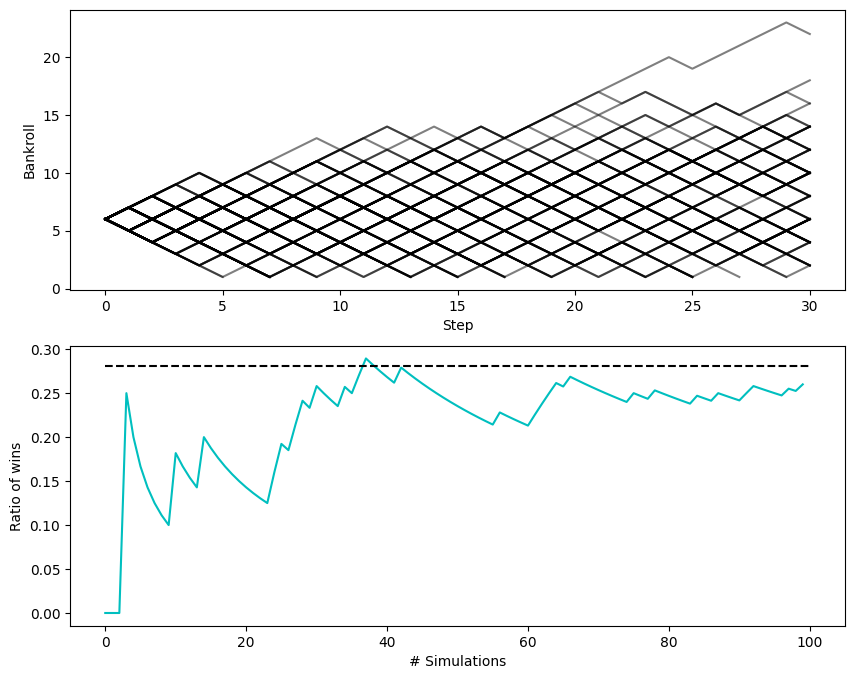
This looks right, although it’s not a clean convergence and I’d feel better with some more testing.

This formula, for “probability of ruin (or non-ruin) before some time T” is actually not one of the usual things explored in first treatments of random walks. We see the “probability of hitting N before 0” a lot, and usually the next one is “probability of hitting \(a\) before \(-b\)”, which I’ve skipped.

Anyway, I’m tempted to move back to betting stuff and talk betting criterion. Or a quick detour on how bookmakers set the odds in a market way. But I’m trying to keep my posts shorter so I’ll stop here for now.

Thanks for reading!