Fractional Kelly

In the previous post, we talked about the Kelly Criterion, a betting strategy that gives the fraction of one’s bankroll to wager to maximize your expected log growth used widely in finance and gambling.

This criterion, at its most vanilla, is

where \(p\) is your assessment of the probability of win, and \(b\) is the offered (fractional) odds upon win. (I’ve omitted a return \(a\) on loss, which makes the formula \(f=p/a - (1-p)/b\), because it is typically \(a=1\) in betting contexts (you lose your wager) and ignored).

This approach is based on our personal assessment of “edge”: how much our belief in the true odds differs from the bookie’s revealed belief captured in \(b\). Which relies on an accurate value of \(p\).

In this post, I want to talk about the fact that: we almost certainly don’t exactly know an accurate value of \(p\)!

I’m going to examine the discussion in this LessWrong post, Never Go Full Kelly and this paper by Baker and McHale. Basically, we use a fraction of the Kelly criterion (“fractional Kelly”) where the fraction is a function of our uncertainty.

I’m not trying to be exhaustive or even didactic, I just wanted to understand this one paper a little better and these are my notes. Maybe it’s useful to someone else also!

Introducing Fractional Kelly

“Fractional Kelly” is the simple idea that instead of wagering \(f\) of our wealth, we wager \(f^*=kf\) of our wealth, with \(0<k<1\). Half-Kelly is \(k=0.5\), for example.

A nice way to see what fractional Kelly implies about your uncertainty, is to frame it in terms of your assessed probability against the bookie’s, of a win, like so:

First note the Kelly criterion involves two values, \(p\) representing your assessment of the event’s probability, and \(b\) representing the bookie’s offered payout. This \(b\) we know captures his assessment of the probability, call it \(q\), and we know \(1/(b+1)=q\) or \(b=(1/q)-1\) (go check out this previous post if that’s unclear).

You can rewrite the criterion in terms of \(q\) instead of \(b\),

Now say we saw \(b\) being offered and wanted to update our initial \(p\) to a new value \(\hat{p}\), with some tradeoff parameter \(k\) capturing our “confidence” in our own assessment vs. the house:

where \(k=1\) means we know everything and the bookie lives under a rock, and \(k=0\) the opposite.

Now notice that using \(\hat{p}\) in lieu of \(p\) in the original criterion leads directly to fractional Kelly:

So in this sense, applying fractional Kelly is exactly the same as applying a tradeoff between your own \(p\) and the bookie’s revealed \(q\).

A framework for fractional

But this doesn’t actually help us quantify our uncertainty, it just reframed it. Let’s say we had some probability distribution over our estimate of \(p\), how could we capture that instead of just taking stabs at point estimates?

Let’s dig through the Baker and McHale paper for their approach.

Recall we are interested in the (log) geometric growth rate of our bankroll,

where \(b\) is assumed fixed. We want to maximize this, and previously, we just let \(p\) be some fixed estimate \(\hat{p}\) (guess, whatever), so we had

Given this single-variable optimization problem, since \(g(\cdot)\) is concave in \(f\) it is sufficient to set the derivative to zero and solve, and we know this yields the classic Kelly criterion.

Now let’s say we keep \(g(\cdot)\) as our goal (expected geometric growth rate), but incorporate some uncertainty in \(p\). Let \(p\) denote the “true” value and let \(Q\) be the random variable representing our estimate, with distribution \(\pi(q)\). (Not to be confused with our use of \(q\) earlier as bookie probability.)

So now we’ve really got a \(p\) and \(b\) both fixed (\(p\) unknown by the way), and a function now over \(q\), \(g(f, q)\). We’d love to average over the distribution of \(Q\) to find our optimal \(f^*\):

This objective function is, in the language of the paper, expected expected utility. But \(f\) itself is a function of \(q\) now, what we are averaging over, so this won’t work.

The paper solves this by just using the standard Kelly formula for \(f\), but introducing a “shrinkage” factor \(k\) on it, and instead of solving for \(f\), solving for \(k\). This leads to:

with \(f(q)=q-(1-q)/b\).

I’m not sure how I feel about this, it feels like we’re not being principled about something. Like I either want to go full Bayesian or just stay frequentist and somehow this seems like neither.

But anyway let’s keep going. Now we’ll look at what that objective function (the integral) looks like.

Finding an optimal shrinkage

The paper implies that solving \(dE/dk=0\) is not possible analytically, best I can tell — it uses numerical methods to look at the plot of the objective function, and it uses a second-order expansion to solve for an approximation of \(k^*\).

Let’s do the plot of the objective function first, their Figure 1. We’ll assume a Beta distribution for \(\pi(q)\), which is very reasonable as this is the standard posterior of a sequence of Bernoulli trials with Beta prior. Note we are parameterizing with mean and variance, not \(\alpha\) and \(\beta\), following the paper.

import matplotlib.pyplot as plt
import numpy as np
from scipy.stats import beta
from scipy.integrate import quad

# define the Kelly betting fraction function f*(q)
def f_star(q, b):
    return ((b + 1) * q - 1) / b

# Expected utility integrand based on Equation (2)
def expected_utility(k, p, b, alpha, beta_param):
    # define the integrand as a function of q
    def integrand(q):
        # beta pdf for q
        pdf = beta.pdf(q, alpha, beta_param)
        # compute f*(q)
        s_val = f_star(q, b)
        # compute the utility: p*ln(1+b*k*f) + (1-p)*ln(1 - k*f)
        return pdf * (p * np.log(1 + b * k * s_val) + (1 - p) * np.log(1 - k * s_val))
    # Numerically integrate from 0 to 1 
    # (this is slow but np.trapz doesn't seem as accurate)
    return quad(integrand, 0, 1)[0]

# Parameters (as in Figure 1: b=1, p=0.7, different sigma values)
p = 0.7
b = 1.0

fig, ax = plt.subplots(1,1, figsize=(7,7))

for sigma in [0.05, 0.1, 0.15, 0.2, 0.25]:
    # compute beta distribution parameters from the paper:
    # alpha = p*(p*(1-p)/sigma^2 - 1), beta_param = (1-p)*(p*(1-p)/sigma^2 - 1)
    variance = sigma**2
    common_term = p * (1 - p) / variance - 1
    alpha_param = p * common_term
    beta_param  = (1 - p) * common_term

    # create a grid of shrinkage coefficients k (avoid k=1 to prevent log(0))
    ks = np.linspace(0, 0.99, 200)
    utilities = [expected_utility(k, p, b, alpha_param, beta_param) for k in ks]

    ax.plot(ks, utilities, color='k', linestyle='-', linewidth=0.5)

ax.set_xlim([0, 1])
ax.set_ylim([-0.25, 0.1])
ax.set_xlabel('Shrinkage coefficient $k$')
ax.set_ylabel('Expected utility (objective func)')

plt.show()

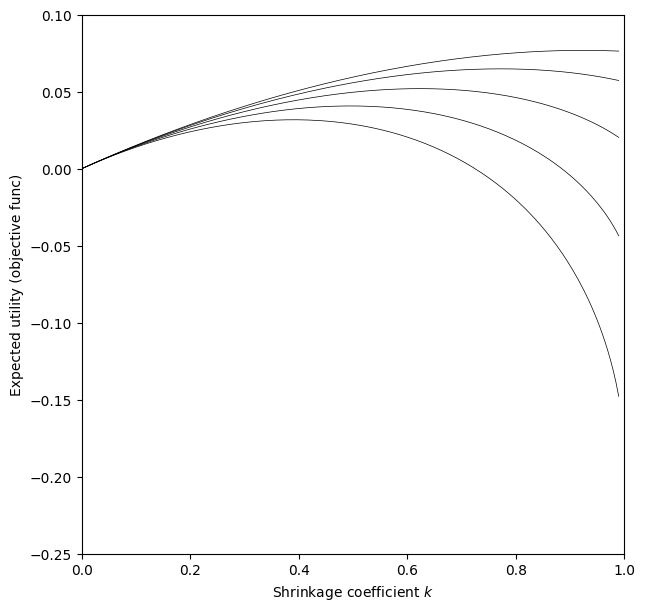
(This nearly exactly matches the paper, although I notice in the paper the higher variance curves curve higher than the low variance ones for low \(k\), whereas ours are strictly decreasing as variance increases.)

The main takeaway from this plot is that as your variance (of \(Q\)) increases, the optimal \(k\) decreases. For \(\sigma=0.2\), optimal is about half Kelly, \(k=0.5\). With \(\sigma=0.05\) however, we are nearly full Kelly.

The paper goes on to actually prove that it is always optimal to shrink, that full Kelly is never optimal, under this model and with a couple stipulations, although without having to specify a distribution of uncertainty. (One important stipulation they get into later is this assumes you have the ability to bet both sides, which isn’t always true. That is if your edge is flipped, you can take the opposite bet.)

Next steps

The paper derives a closed form expression for an approximation of \(k^*\) using a second-order expansion of the expected utility objective function, which I’d like to check but will leave for a separate post. The LessWrong post also makes a nice connection to the Sharpe ratio which I’d like to dive into later.

For now though let’s call it a day. Thanks for reading!