Betting strategies and the Kelly Criterion

In the last couple posts we’ve been looking at some basic concepts in probability theory from the standpoint of betting. First, we reviewed how odds, probability, and bets are connected, and then we looked at the random walk behavior of a gambler’s bankroll over time making bets.

In this post, we’ll look at basic betting strategy and the Kelly Criterion.

Basic idea

The odds (and therefore payoff) is set by a bookmaker, and so it’s based on his assessment of the probability of a win. Setting aside vig for a sec, recall odds \(D\) imply the bookmaker thinks the probability is \(1/D=p\). (So for example, odds of \(D=4\) imply a chance of the event happening with probability \(p=1/4=0.25\) and carry a payout of \(D-1=3\) (in addition to getting your 1 dollar bet back).)

Now consider two scenarios:

• If we also think the probability is \(1/D=p\), then we shouldn’t make the bet. We have no edge, so our expected return is 0.

• If we think the probability is not \(p\), then we (think we) know something the bookmaker doesn’t, and we are in a position to bet. This is our “edge”. Denote our probability as \(p\) and the bookie as \(p'\). If our \(p\) is greater than the bookie’s \(p'\), then we should take the bet — our EV is positive. And if \(p < p'\) we should bet against the thing happening (for example on the other team winning).

That’s really it. So then the question is, how much should we wager when we think we have an edge?

Naive strategy

Let’s say we have access to the true probability of win, and the bookie only has a noisy estimate. So we always have an “edge”. But we don’t know any better and so we just do a full unit bet every time, regardless of the payout offered.

Let’s see what that looks like.

import matplotlib.pyplot as plt
import numpy as np

np.random.seed(316)

N, m = 50, 100      # num runs, num bets
b = 1               # initial bankroll

# generate TRUE probabilities
probs = np.random.uniform(0.1, 0.9, size=(N, m))

# generate noisy bookie probabilities and make sure variance doesn't take us past [0,1]
book_probs = probs + np.random.normal(0, 0.05, size=(N, m))
book_probs = np.clip(book_probs, 0.01, 0.99)

# compute the payouts
payouts = 1 / book_probs

# generate outcomes
mask = np.random.uniform(0.1, 0.9, size=(N, m)) < probs
outcome = np.where(mask, payouts, -1)

# compute cumulative bankroll
bank = b + np.cumsum(outcome, axis=1)

fig, ax = plt.subplots(1,1, figsize=(10,5))
for i in range(N):
    ax.plot(range(m), bank[i,:], 'k-', alpha=0.4)
ax.axhline(y=0, color='r', linestyle='--')
plt.show()

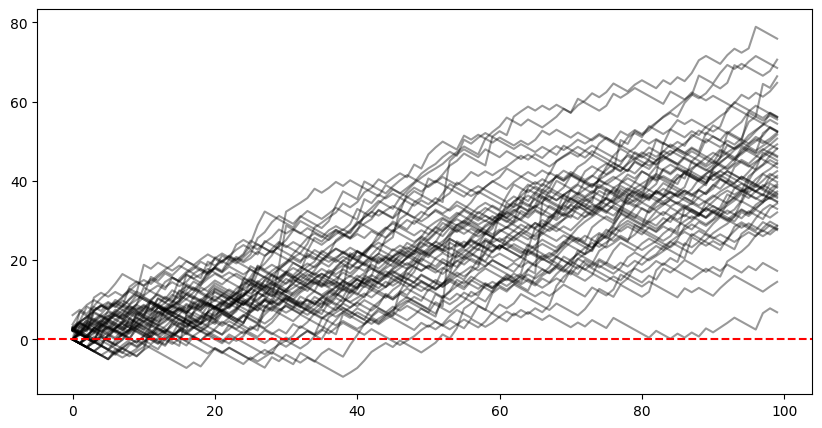
(Please note I set the true probabilities to between 0.1 and 0.9 to prevent crazy jumps (a very unlikely event will have a huuuuge payoff and you get gigantic jumps up or down) — this was because most events you can gamble on aren’t so one-sided, but it’s certainly a possible in other places.)

A couple observations off this naive approach:

• We have, casually speaking, an upward drift, as we tend to win, on average, in the long run.
• But despite our average drift upwards, We are still subject to ruin.
• Also, despite our exposure to ruin, we haven’t increased our wagers when we have a big edge, so our gains are overly modest.

Kelly Criterion

We should find a way to cleverly adjust the amount of our bet to be somehow proportional to how much our edge is, and do so in a way that maximizes growth but also prevents ruin.

John Kelly, a researcher at Bell Labs, described a criterion in the 1950s that sizes your bets in a way that maximizes the long-term expected value of the (log) of your bankroll.

Call your personal assessment of the probability of an event \(p\). Let \(b\) represent the proportion of your bet gained with a win — note this is fractional odds, so it implies a bookie probability of \(1/(b + 1)\).

Kelly’s criterion says to wager a fraction \(f\) of your bankroll equal to:

Notice a few properties of this simple formula:

• In order for \(f\) to be positive (\(f>0\)), we need \(p > (1-p)/b\) which is \(p/(1-p) > 1/b\). This means my perceived odds (\(p/(1-p)\)) are greater than the bookie’s perceived odds (\(1/b\)).

• If your odds/probability are the same as the bookie’s (no edge), then \(p = 1/(b+1)\) and this gives \(f=0\). (Check by substituting in \(1/(b+1)\), or for a little easier algebra, put in \(b=(1-p)/p\).)

• If your odds are lower than the bookie’s, you’ll get \(f<0\) and the criterion would encourage you that you still have an edge, just take the other side of the bet!

Let’s try plotting this surface, of the Kelly criterion value given our \(p\) vs bookie’s \(p'\).

def f(p1, p2):
    return p1 - (1-p1)/((1-p2)/p2)

a, b = 0.1, 0.9
p1 = np.linspace(a, b, 100)
p2 = np.linspace(a, b, 100)
P1, P2 = np.meshgrid(p1, p2)
F = f(P1, P2)
F2 = f(1-P1, 1-P2)

# create f where we swap sides of the bet when our p < less than bookie p
Fs = np.where(P1 < P2, F2, F)

fig, ax = plt.subplots(1,1, figsize=(8,6))
c = ax.contourf(P1, P2, Fs, levels=np.linspace(0, 1, 50), cmap='Blues')
ax.plot([a, b], [a, b], color='r', linestyle='--', zorder=100)
ax.set_xlabel('Our $p$')
ax.set_ylabel('Bookie $p$')
cb = fig.colorbar(c, ax=ax, ticks=np.linspace(0, 1, 11))
cb.ax.set_yticklabels(['{:.1f}'.format(i) for i in np.linspace(0, 1, 11)])
plt.show()

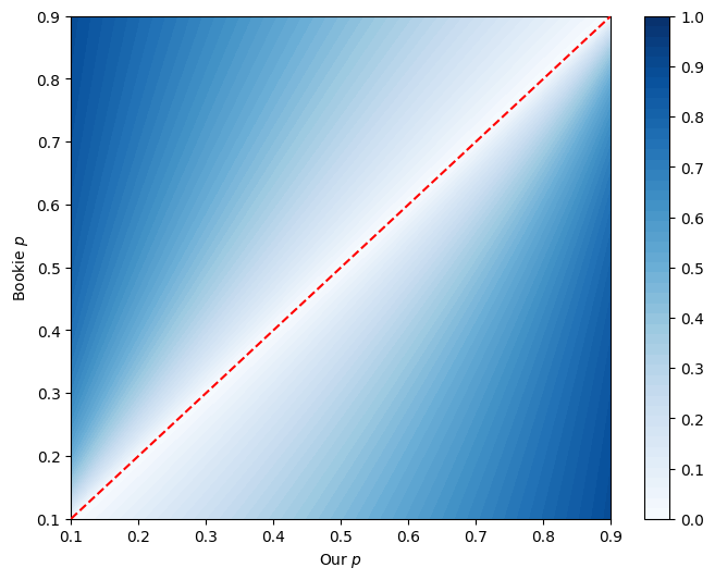
Note that above the red line, we need to swap our bet. So like if we thought the event had a 20% chance of win, and the bet offered implied a 80% chance of win, then we’d take the odds on it losing (where everything flips and we’re 80% sure against his 20%), with a high \(f\).

(Again I set probabilities in \([0.1, 0.9]\) because at 0 and 1 we get some divide by zero.)

Now let’s test a straightforward application of the Kelly bet to our gambler’s walk from before, where we again give the bookie a noisy estimate of probability.

np.random.seed(311)

N, m = 50, 100      # num runs, num bets
b = 1               # initial bankroll

fig, ax = plt.subplots(1,1, figsize=(10,5))

for i in range(N):
    # generate TRUE probabilities
    probs = np.random.uniform(0.1, 0.9, size=m)

    # generate noisy bookie probabilities and make sure variance doesn't take us past [0,1]
    book_probs = probs + np.random.normal(0, 0.05, size=m)
    book_probs = np.clip(book_probs, 0.01, 0.99)

    # generate probabilities of actual outcome
    outcome = np.random.random(m)

    # ----> compute the Kelly bet proportions
    fs = f(probs, book_probs)

    bank = b + np.zeros(m)
    for j in range(m-1):
        bet = 1 / book_probs[j]  # this is decimal odds = win includes wager
        p1, p2 = probs[j], book_probs[j]
        fj = p1 - (1 - p1) / ((1 - p2) / p2)
        wager = fj * bank[j]

        # subtract off wager regardless of outcome
        bank[j+1] = bank[j] - wager
        if outcome[j] < probs[j]:
            # we win, we get wager + payoff
            bank[j+1] += wager * bet
    
    ax.plot(range(m), bank, 'k-', alpha=0.4)

ax.axhline(y=0, color='r', linestyle='--')
ax.set_ylim([-1, 10])
plt.show()

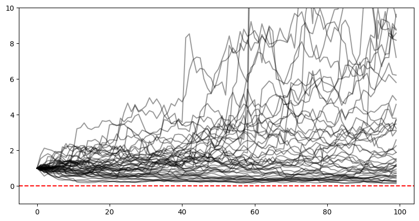
So we’ve got a ton of runs asymptotically reaching ruin, a few glorious runs that literally go off the chart, but one thing to note is that we never actually hit ruin. This is because (obviously) we’re always only betting a fraction of our bankroll.

We could in theory have a Kelly fraction of 1 (bet your entire bankroll), but this only happens when our \(p=1\) which does not happen in reality. So with Kelly in \((0,1)\), we will never go all in and can never hit ruin.

That said, typically you don’t go “Full Kelly” and bet the entire proportion.

Let’s try to better understand why Kelly is what it is and then come back to this.

Deriving Kelly

To understand how to use Kelly I think it’s important to understand it’s derivation. I’ll walk through the standard informal derivation (for example see Wikipedia or here) but add a good bit of commentary that feels helpful to me.

Start with \(X_0\) of bankroll and bet a fraction \(f\) of that on an outcome that occurs with probability \(p\) (let \(q=1-p\)) and offers odds of \(b\) for a win. Let’s also pretend we have odds of \(a\) for a loss — in a normal gambling setting, typically \(a=1\) (we just lose whatever we wagered), but in other settings (say, finance), we may have a lopsided upside/downside situation, so we’ll keep this in for generality in the derivation.

Recall this \(b\) (and \(a\)) represents fractional odds. So if have 1, and we wager 1 on odds of \(b=2\) (aka 2:1 against, aka implied probability of 33%), we gain 2 plus our wager back, and we’re at 3 total. If we lose, with \(a=1\), we’re at 0. With \(a=2\), we lose double our wager and we’re at -1!.

Similarly, if we have 1, and we wager 0.5 on the same odds, we gain \(2\times 0.5 = 1\) plus our wager back and we’re at 2 total (if we lose, for \(a=1\), we’re at 0.5). Etc.

So to put this another way (yes I realize this might feel pedantically repetitive, that’s the idea), with starting bankroll \(X_0\), after your first bet, w.p. \(p\) we have \(X_1 = X_0 + (f X_0) b = X_0(1 + fb)\). After your second bet, with another win, you have \(X_2 = X_1(1+fb) = X_0 (1+fb)^2\), etc. (Note we’ve made the simplifying assumption that \(b\) and \(f\) are the same in every step.)

For losses we have the same thing: after one loss, \(X_1 = X_0 - (f X_0) a = X_0 (1 - fa)\), after two losses, \(X_2 = X_0(1-fa)^2\), etc.

Getting an expression for bankroll at time \(t\)

Putting them together, with \(n_w\) our number of wins and \(n_l\) our number of losses, we have

As \(t\rightarrow\infty\), by the law of large numbers this becomes

(where \(q=1-p\)). Let’s take logs

and note we’d like

which is the same as maximizing the geometric rate, which we’ll revisit in a second.

Solving for optimal \(f\)

For now, to solve this single-variable optimization problem, we note the objective function is concave over \(f\) and so just need to set the derivative to zero and solve:

Voila. When \(a=1\) this is what we said earlier.

Connection to geometric rate

We’ve mentioned Kelly is often defined as maximizing expected geometric growth. Why?

“Geometric growth” is the discrete interval version of “exponential growth”, and is defined as

This should be familiar: with \(r<1\), this represents the growth of \(X_t\) as it experiences an increase of \(r\) in every period \(t\), with a starting value of \(X_0\).

Equating this to our slightly more complicated situation before, we have

so we could define \(r' = (1+fb)^p (1-fa)^q\) as our rate, and then our optimization from before amounted to \(\text{arg}\max_f r'\). That is, we are maximizing the expected geometric growth rate.

Flirting with Full Kelly

Before we stop, I want to highlight that \(f^*\) maximizes the expected geometric growth. Let’s plot what this looks like for different values of \(b\) and with a fixed \(p=0.6\).

fig, ax = plt.subplots(1,1, figsize=(8,8))

true_p = 0.6
book_ps = np.arange(0.3, 0.8, 0.1)
colors = plt.cm.Blues_r(np.linspace(0, 1, len(book_ps)))

for i, book_p in enumerate(book_ps):
    b = (1-book_p)/book_p

    xs = np.linspace(0, 0.9, 100)
    ys = true_p * np.log(1 + xs * b) + (1 - true_p) * np.log(1 - xs)

    ax.plot(xs, ys, color=colors[i], label=book_p)

ax.legend([f'{bp:.1f}' for bp in book_ps])
ax.axhline(0, color='black', linewidth=0.5)
ax.spines['top'].set_visible(False)
ax.spines['right'].set_visible(False)
ax.spines['bottom'].set_visible(False)
plt.show()

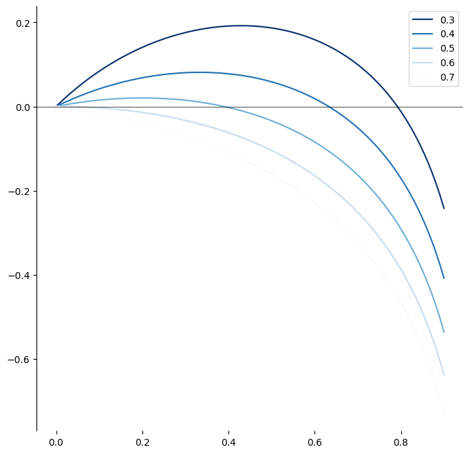
Expected growth on the \(y\) axis, Kelly fraction on the \(x\) axis — You can visually see the maximum, and as our edge decreases we’re forced closer to 0.

However, using this maximizing fraction, the “full” Kelly amount, is overly aggressive for most people in most cases.

If someone offered you even-money on something you thought was a 60% chance, the Kelly criterion would have you stake \(0.6 - 0.4/1=0.2\) aka 20% of your entire bankroll (see above graph). Would you actually stake a fifth of your entire bankroll on something you thought only had a 60% shot to begin with, regardless of your edge? Probably not.

So you typically do “fractional” Kelly.

This runs into a whole new messy world: how will we model our uncertainty about our own and our bookmaker’s probabilities, how will we model our risk tolerance, etc. This LessWrong post starts to do a deeper look, and I’d like to take my own foray into this, but that’s enough for one post.

Thanks for reading!