Blessing of Dimensionality: Manifold Learning of Random Walks

I was playing around with UMAP recently and noticed that when you have a random walk in high dimensions, it resolves to a simple line in the UMAP-generated 2-dimensional projection. This follows intuitively from how UMAP works, by creating a low-dimensional representation that closely captures the fuzzy topological structure of the data in its original dimension — the steps of the random walk are close together, so the algorithm connects them, and when you get into high dimensions they have “room to breathe” so the algorithm doesn’t also accidentally connect non-consecutive ones.

In this sense, UMAP seems to benefit from a kind of “blessing of dimensionality”. The extra dimensions help it suss out structure. And since all manifold learning algorithms do a superficially similar process, of learning local structure and mimicking it in the lower-dim space, I’m curious if this happens with other methods. It is pretty standard to show manifold learning algo’s ability to capture crazy data topologies, but I thought the behavior with RWs was the cleanest example of how these methods actually seem to need more dimensions to infer structure.

Anyway, I wanted to explore this observation a little more in a post, for posterity and in case it’s interesting to anyone else. This is not a terribly serious post, and I think the more deep connection would be to explore how this connects to kernels, but here we go.

Introductions

Hi, I’m a Manifold Learner

Uniform Manifold Approximation and Projection (UMAP) is a technique for dimension reduction introduced in 2018 with this paper by the great Leland McInnes. It is in the class of manifold learning/dim reduction techniques with other famous methods like t-SNE and isomaps. UMAP is (I gather) the method of choice in the bioinformatics field, and the paper’s 15k+ citations indicate it’s quite popular in general usage too. Of note, t-SNE and isomaps both have implementations in Python’s popular scikit-learn package, while UMAP is a standalone package with (in my humble experience) a little more finnicky dependencies, so you often find t-SNE a more common choice. But the UMAP docs are wonderful, so check it out if you haven’t.

Without getting into the algebraic topology and category theory that underlies how UMAP works, which I don’t understand (but would love to), the gist of how it works is that it first finds a (fuzzy) topological representation of the data that sort of connects nearby points, with “nearby” defined in a locally scaling way, and then it finds a low-dimensional embedding of the data that optimizes its fidelity to this representation in terms of the cross-entropy.

For us visual learners, here’s what that fuzzy topological representation looks like for some points generated along a sine curve: (image lifted from the docs)

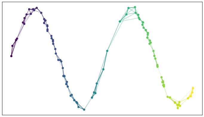
And the corresponding 2-d embedding would be some sort of straight line.

t-SNE (t-distributed Stochastic Neighbor Embedding) is very similar to UMAP in that it learns local structure and attempts to optimally mimic this in a lower-dimensional setting, but instead of learning topological structure, it uses a probabilistic sense of structure: what are the Gaussian joint probabilities in the original space, and let’s replicate that with Student t-dists in the embedded space.

There are many others: kernel PCA (which is like the linear projection of PCA but in a kernel space that enables non-linear projections), isomaps, locally linear embeddings, etc.

Nice to meet you, I’m a Random Walk

A “random walk” is a class of stochastic processes consisting of series of successive steps over some space, with each step a random sample from some distribution.

As a basic example, consider the sequence defined by \(\mathbf{x}_{t+1} = \mathbf{x}_t + \varepsilon_t, \quad \varepsilon_t \sim \mathcal{N}(\mu, \Sigma)\)

At every time step, we generate our next move from a multivariate Gaussian with mean \(\mu\) and covariance \(\Sigma\). This usually generates something looking like this:

In the limit, this becomes a Wiener process and describes Brownian motion, a model for the movement of a tiny particle suspended in liquid. These are very fundamental objects and so many many volumes have been written about it, which we won’t attempt to summarize here.

Let’s just see what happens when we mix these two ideas together — let’s generate a RW in high-dimensional space and find the low-dim projection of it using UMAP.

High-dim RW to low-dim manifold

import warnings
warnings.filterwarnings('ignore')

import matplotlib.pyplot as plt
import numpy as np
import umap

np.random.seed(317)

ds = [2, 3, 10, 100]
N = 50

fig, axs = plt.subplots(2,4, figsize=(12,6))

for i,d in enumerate(ds):
    steps = np.random.multivariate_normal(np.zeros(d), np.eye(d), size=N)
    walk  = np.cumsum(steps, axis=0)
    walk_u = umap.UMAP().fit_transform(walk)

    axs[0,i].scatter(walk[:,0], walk[:,1], s=30, c='k', zorder=100)
    axs[0,i].plot(walk[:,0], walk[:,1], 'k-', alpha=0.2)
    axs[1,i].scatter(walk_u[:,0], walk_u[:,1], s=30, c='c', zorder=100)
    axs[1,i].plot(walk_u[:,0], walk_u[:,1], 'c-', alpha=0.2)
    axs[0,i].set_title(f'd = {d}')

plt.tight_layout()
plt.show()

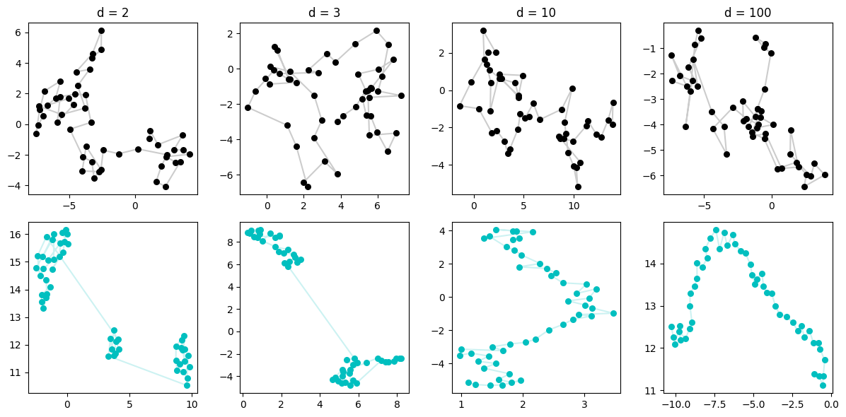
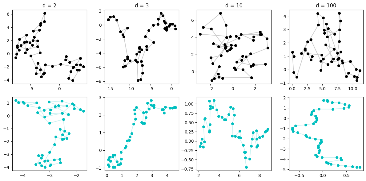
This is really neat. When the RW is in \(d=2\), the sequence overlaps itself and so we can imagine the fuzzy weighted k-neighbors type graph that UMAP makes is confused by who should be connected to who. (whom?) So it finds some clustering which, admittedly, does happen to exist in the original data, but doesn’t magically discover the points are in a sequence.

We then progress to higher dimensions, and please note that our plots are only showing the first two dimensions — basically the shadow on the ground of what the data looks like. But in reality, these points are very spread out across increasingly more dimensionality. This means, that although we can’t see it, we can imagine that the only points that are close, are points that are consecutive! If not, you’d never happen to be close by the curse of dimensionality — which in this case is kind of a blessing!

So UMAP is increasingly able to discover the points are fundamentally situated along a single line, and so when it constructs a low-dimensional manifold, it mimics that.

We might wonder, will the high dimensionality allow any set of samples to resolve to a line? We would think not, because we lose that fact of “only consecutive points are close”, but let’s check by sampling directly from a Gaussian, no steps.

np.random.seed(314)

ds = [2, 3, 10, 100]
N = 50

n_components = 2
n_neighbors  = 15   # default 15
min_dist     = 0.1  # default 0.1

fig, axs = plt.subplots(2,4, figsize=(12,6))

for i,d in enumerate(ds):
    data = np.random.multivariate_normal(np.zeros(d), np.eye(d), size=N)
    data_u = umap.UMAP(
        n_components=n_components,
        n_neighbors=n_neighbors,
        min_dist=min_dist,
    ).fit_transform(data)

    axs[0,i].scatter(data[:,0], data[:,1], s=30, c='k', zorder=100)
    axs[0,i].plot(data[:,0], data[:,1], 'k-', alpha=0.1)
    axs[1,i].scatter(data_u[:,0], data_u[:,1], s=30, c='c', zorder=100)
    axs[1,i].plot(data_u[:,0], data_u[:,1], 'c-', alpha=0.1)
    axs[0,i].set_title(f'd = {d}')

plt.tight_layout()
plt.show()

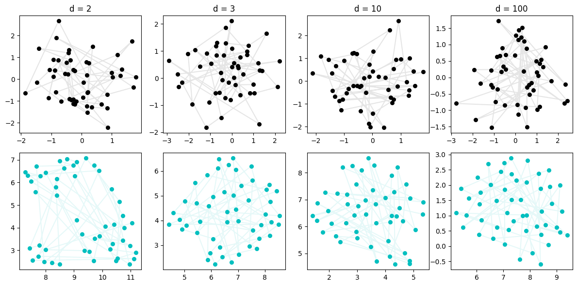
Okay good — we seem to verify our intuition that this low-dim line shouldn’t emerge when our data is truly evenly sampled. Close points (in time) are not necessarily close (in space) and so UMAP sees the same thing we do: a blob.

What else can we wonder about?

Let’s try two

How about two random walks in the same space? We’d think that the same thing will happen: for low-dimension, UMAP will be unable to separate them, but in high-dim, each line will have enough of its own “space” for UMAP to discover the line-like low-dim manifold that best mimics their behavior.

np.random.seed(317)

ds = [2, 3, 10, 100]
N = 50

fig, axs = plt.subplots(2,4, figsize=(12,6))

for i,d in enumerate(ds):
    walks = []
    for k, color in zip([0,1], ['k', 'g']):
        steps = np.random.multivariate_normal(np.zeros(d), np.eye(d), size=N)
        walk  = np.cumsum(steps, axis=0)
        walks.append(walk)
        
        axs[0,i].scatter(walk[:,0], walk[:,1], s=30, c=color, zorder=100)
        axs[0,i].plot(walk[:,0], walk[:,1], color=color, linestyle='-', alpha=0.2)
    
    walks = np.vstack(walks)
    walk_u = umap.UMAP().fit_transform(walks)

    axs[1,i].scatter(walk_u[:,0], walk_u[:,1], s=30, c='c', zorder=100)
    axs[1,i].plot(walk_u[:N,0], walk_u[:N,1], 'c-', alpha=0.2)
    axs[1,i].plot(walk_u[N:,0], walk_u[N:,1], 'c-', alpha=0.2)

    axs[0,i].set_title(f'd = {d}')

plt.tight_layout()
plt.show()

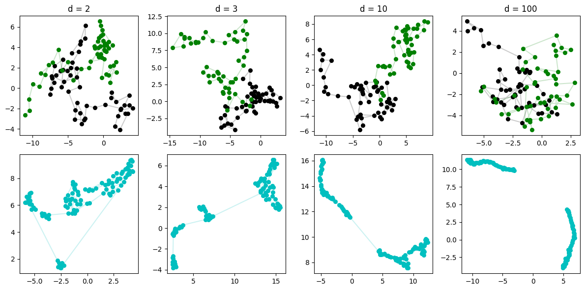
Very cool. Even with two RWs, by the time we get to \(d=100\), it’s quite easy for UMAP to suss out that there are two separate very 1-dim manifolds-worth of data, the two lines.

Checking out the other guys

Earlier we mentioned other manifold learning techniques. The other highly popular method is t-SNE. How does it do with this problem? It’s very clean and we’d expect similar results.

from sklearn.manifold import TSNE

np.random.seed(317)

ds = [2, 3, 10, 100]
N = 50

fig, axs = plt.subplots(2,4, figsize=(12,6))

for i,d in enumerate(ds):
    steps = np.random.multivariate_normal(np.zeros(d), np.eye(d), size=N)
    walk  = np.cumsum(steps, axis=0)
    walk_u = TSNE().fit_transform(walk)

    axs[0,i].scatter(walk[:,0], walk[:,1], s=30, c='k', zorder=100)
    axs[0,i].plot(walk[:,0], walk[:,1], 'k-', alpha=0.2)
    axs[1,i].scatter(walk_u[:,0], walk_u[:,1], s=30, c='c', zorder=100)
    axs[1,i].plot(walk_u[:,0], walk_u[:,1], 'c-', alpha=0.2)
    axs[0,i].set_title(f'd = {d}')

plt.tight_layout()
plt.show()

Before this turns into an sklearn docs page, we can see that t-SNE performs similarly. (And, I won’t show it here but it also performs similarly on the two-walk case.)

This is all reassuring, that any of these manifold methods are able to capture the simple local structure of a random walk in their 2-d embedding — but again, interesting to me that for all methods, their performance increases with the dimensionality.

Other thoughts

The idea that the higher dimensions are not only handled well by manifold learning algorithms, but actually beneficial to them, seems very interesting. I’m curious if there’s some other structure (other than random walk) that might demonstrate this, and (even better) if you could demonstrate it theoretically.

This also seems closely tied to the whole idea of kernels, and projecting data into a space with more dimensions to work with, doing your classifier or whatever there, and then projecting back.

Hope this was interesting, thanks for reading.