Python class for Hawkes processes

Written on June 26th, 2017 by Steven Morse

This post is about a stochastic process called the Hawkes process. I offer some Python code for generating synthetic sequences and doing parameter estimation, and also cover some theoretical preliminaries.

I am using the Hawkes process in some on-going research — I found that it is popular enough to have a large, interdisciplinary literature, but specialized enough that the available software packages are few and far between. At the end of this blog, I link to several repos already out there for this family of models. They are high quality, production-level packages, and miles beyond what I offer here, but are in my opinion overkill for someone just getting started and needing some basic code to fiddle with.

I’m hoping to bridge this gap by offering both a beginner-friendly math exposition and an immediately useable, if relatively basic, code library in Python.

Prelims

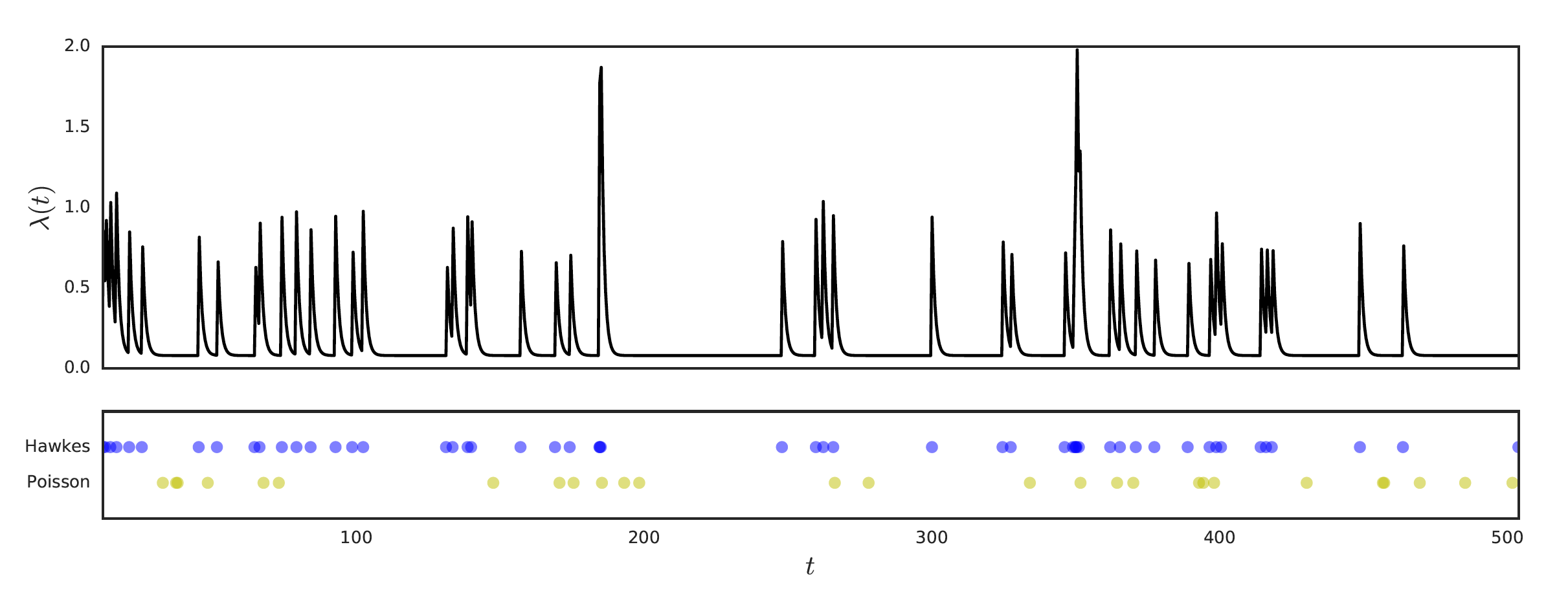
We can define a point process as a random and finite series of events governed by a probablistic rule. For example, the ubiquitous Poisson process is a series of points along the nonnegative real line such that the probability of \(k\) points on any interval length \(n\) is given by a Poisson distribution with parameter \(\lambda n\). The bottom series of points in the figure above is an example of a Poisson process (with rate \(\lambda=0.1\)).

We may even consider a \(U\)-dimensional Poisson process, with \(U\) different Poisson processes generating events in \(\mathbb{R}^U\), each with a different rate \(\lambda_u\). Now, the overall number of points in a particular interval (or now more appropriately, volume) is again given by a Poisson distribution with parameter \(\lambda n\), where the rate \(\lambda = \lambda_1 + ... + \lambda_u\) (the Poisson superposition theorem). This additive property allows us to compute the probability that a particular event originated from a particular dimension \(u_i\) as \(\lambda_{u_i} / \lambda\).

You can also show that the number of events in disjoint subsets are independent of each other. This leads to the critical observation that the Poisson process is memoryless. Another way to state this is that the interarrival time between two successive events is an exponential random variable, and therefore the probability of the next interarrival time is independent of the previous. This memoryless property makes the Poisson process an extremely tractable modeling tool.

Hawkes process

However, the memoryless property of Poisson processes means that it is unable to capture a dependence on history, or in other words, interaction between events. For example, we may want the event of an arrival to increase the probability of arrivals in the next small interval of time.

For this, we introduce the Hawkes process, which gives an additive, decaying increase to the intensity function for each new arrival. Now, the intensity function is only conditionally Poisson: that is, given the history of events \(\{t_i\}\) up to \(t\), the conditional intensity at \(t\), that is \(\lambda(t ; t_i < t)\), is Poisson.

Definition. Hawkes process. Consider a sequence of events \(\{(t_i, u_i)\}_{i=1}^n\) consisting of a time \(t_i\) and dimension \(u_i\) (i.e. the \(i\)-th event occurred at time \(t_i\) in dimension \(u_i\)), for \(t_i\in\mathbb{R}^+\) and \(u_i\in \mathcal{U}=\{1,2,...,U\}\). This sequence is a Hawkes process if the conditional intensity function has the parameterized form

\[\lambda_u (t; \Theta) = \mu_u + \sum_{i:t_i < t} h_{uu_i}(t-t_i; \theta_{uu_i})\]

where \(\Theta=(\mu, \theta)\) are the model parameters and \(H=[h_{ij}]\), \(h_*(t):\mathbb{R}^+ \rightarrow \mathbb{R}^+\) is the matrix of triggering kernels (also sometimes called the excitation function or decay kernel) which is varying with \(u\) and \(u_i\).

In other words, imagine \(U\) streams of events, all happening simultaneously. And imagine that, within a stream \(u\), any previous event \(t_i\) has the capability of increasing the likelihood of a future event occurring at time \(t\), according to some function \(h_{uu}(t-t_i)\) which we control with parameters \(\theta_{uu}\). Further, imagine that streams can influence not only themselves, but also each other, according to the same function, and parameters \(\theta_{u_i u_j}\) (for the effect of stream \(j\) on \(i\)).

We’d like to model the triggering kernel \(h(\cdot)\) as something that decays with time: as previous events become more and more distant, they have less and less effect on the present. A natural choice is the exponential function \(h(t)=\omega e^{-\omega t}\). We may also separate the exponential function itself from a scaling factor, so we write:

\[h_{uu'}(t) = \alpha_{uu'} \omega_{uu'} e^{-\omega_{uu'} t}\]

and we might even set \(\omega_{uu'} = \omega\) globally, and only tune the \(\alpha\)’s (which still gives us \(U^2+U+1\) parameters to learn).

An example

A univariate example is given above, and compared to a Poisson process with the same base rate \(\mu\). In the Hawkes process, we see that events cause a spike in the intensity \(\lambda(t)\), which frequently leads to more events, more spikes … this results in a burst of activity (which happens to well-model the actual way many event sequences behave, such as the communication habits of people).

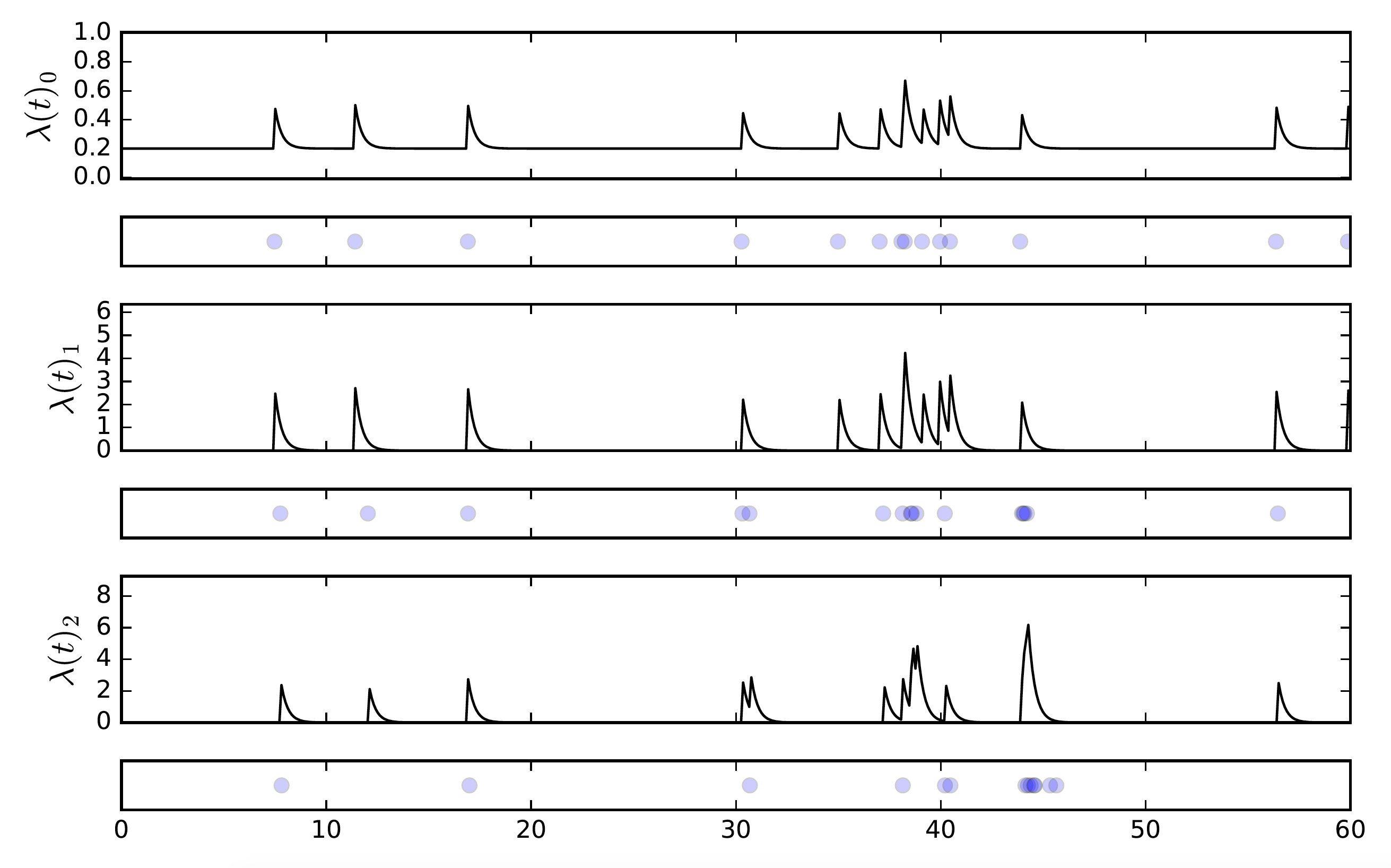
In the multivariate example above, we have 3 different streams of events, call them \(e_0\), \(e_1\), and \(e_2\). We have engineered it by setting the parameters such that \(e_0\) has an influence on itself and \(e_1\), and \(e_1\) has an influence on \(e_2\). We also set the background rate to zero for all the streams except for \(e_0\) — this way, if we see an event on \(e_1\) or \(e_2\) we know it came from a previous event on the parent stream, not a random event.

This creates a cascading effect that we see almost immediately: a background event in \(e_0\) causes a “child” event in \(e_1\), which then leads to a child event in \(e_2\). Notice that in the second cascade, there is no event in \(e_2\) even though it experienced a spike in probability of an event happening. Because \(e_0\) is self-exciting, we see temporal clustering there which translates to bursts in its child processes.

Generating synthetic sequences

How did we generate the data in the figures above? A well-worn approach is known as Ogata’s thinning method, which essentially generates new events from an exponential distribution parameterized by the Hawkes intensity at that time, but then rejects some events with some probability that decreases as the time since the last event increases.

In the multivariate case, this is only slightly more complicated, since we must also attribute each generated event to a particular dimension based on the proportional likelihood the new event came from that dimension. In expositions like this excellent slide deck, these two steps are called Reject-Attribute.

The details are apparent in the repo, but let us mention two important modifications.

The algorithm as typically described requires \(O(n^2 U^2)\) operations to draw \(n\) samples over \(U\) dimensions, which is prohibitive for large \(n\) or \(U\). Instead, we modify an approach mentioned in this paper. Given the rates at the last event \(t_k\) (which note do not include effects of \(t_k\)), we can calculate \(\lambda(t)\) for \(t>t_k\) by

\[\lambda_u(t) = \mu_u + e^{-\omega(t-t_k)}\big(a_{uu_k} \omega + (\lambda_u(t_k) - \mu_u)\big)\]

which we can do in \(O(1)\), and only requires saving the rates at the most recent event. Note also that when \(0 < t-t_k < \epsilon\), this reduces to

\[\lambda_u(t) = \lambda_u(t_k) + a_{uu_k} \omega\]

or in other words, the previous rate plus the maximum contribution the event \(t_k\) can make since it has just occurred.

Secondly, we find that texts describing the algorithm typically frame the attribution/rejection test as finding an index \(n_0\) such that a uniformly random number on \([0,1]\) is between the normalized successive sums of intensities around that index. But note that this entire procedure amounts to a weighted random sample over the integers \(1,2,...,U+1\) where the probabilities are the normalized rates, and selecting \(U+1\) is equivalent to the “rejection” condition. This allows us to use optimized package software for weighted random samples, instead of something like a for-loop (as is present in even production-level Hawkes process software, like the hawkes package in R see below).

Parameter estimation

Lastly, we will mention a few approaches for estimating the parameters of a Hawkes process. It would be impossible to reasonably cover the entire literature, or even a single method, in any depth here, but I’ll try to cover the major “streams” (haha) of technique (including the approach I take in the repo’d code).

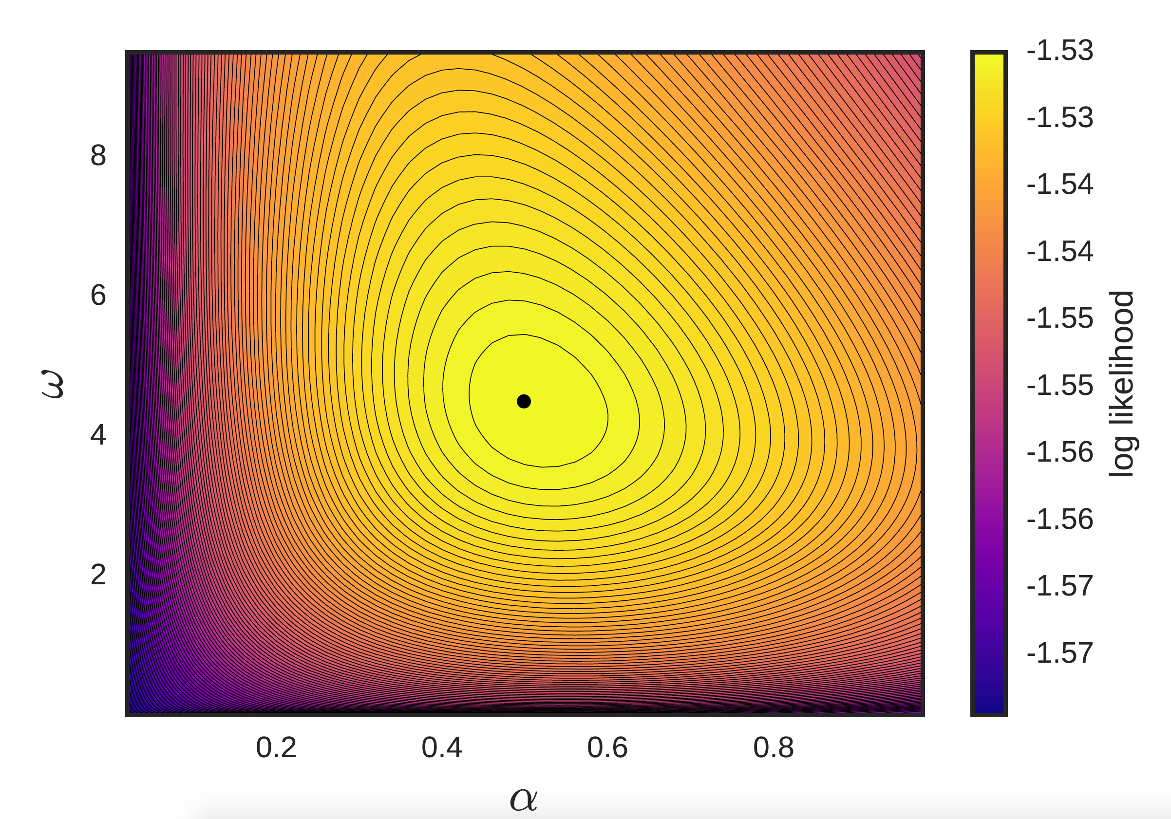
• Maximum-likelihood estimation (MLE). We can actually express, in closed-form, the (log) likelihood of the data under a choice of parameters. As a result, we can simply do something like \(\textrm{max} \mathcal{L}(\Theta)\) for log-likelihood function \(\mathcal{L}\), applying some appropriate optimization machinery of our choosing (e.g. in the univariate case where we also have the 1st and 2nd order gradients, we have endless options). However, in practice the log-likelihood is extremely flat near the optimum, leading to slow convergence, degenerate Hessians, etc. (See figure below.)

The sheer number of parameters also leads to massive overfitting and problems of sparsity. As a result, most methods apply some type of regularization (typically on the \(\alpha\)’s), such as an L2-norm (here), or L1-norm and nuclear norm (here), etc.

• Bayesian frameworks. We can achieve this regularization instead by placing a prior on the various parameters. This paper places a Gamma prior on the scaling parameters \(\alpha_{uu'}\), a log-normal prior on the triggering kernel params \(\omega_{uu'}\), etc., and uses a collapsed Gibbs sampling procedure.

• Expectation-maximization (EM). In the univariate case, where sparsity is not a concern but the challenges of MLE persist, many apply EM. Briefly, EM is designed to estimate parameters when there is missing data. It takes a guess at the missing entries based on the current parameter estimate, then re-estimates the parameters using these guesses, then iterates.

  In the Hawkes application, our missing data is the unknown matrix of which event caused some subsequent event. That is, each observed event is either a parent (i.e. a background event), or a child (i.e. result of some excitation from a previous event). By incorporating this magic, completely unknown knowledge, we suddenly add a lot of structure to the problem that helps stabilize parameter estimation. (As a bonus, we get an estimate of the parent-child relationships of each event, although I have not seen research making use of this byproduct.)

  Some papers using this approach in seismology, email data (with a nice exposition), and a nonparametric version (with a tie-in to gradient descent). There are many others.

  Extended to the multivariate case, this comes up as majorization-minimization in this paper.

• Maximum aposteriori (MAP) EM. We can incorporate some regularization into the EM framework by introducing a prior and doing MAP EM. This is a simple extension of the EM methods, but allows us to reasonably estimate in the multivariate case. It is our methodology in this preprint, where we apply the process to individual credit card purchase activity. I also talk about it in my masters thesis here.

This repo includes this MAP EM approach. It is not very sophisticated: it treats \(\omega\) as a global hyperparameter, does not incorporate a prior on the background rates \(\mu\), and I think the expression I am using for the “complete data log-likelihood” in the multivariate case is actually a tight lower bound on the real value as they show here.

Hopefully it is helpful/interesting to you! Please consider citing our preprint if you find the MAP EM approach useful to your own research. Feel free to send any feedback/questions, via Twitter or an email (see my about page).

Further resources

Some of what’s out there, that I’ve found:

• Tick is a Python library for statistical learning of point processes, with some additional optimization toolkit tools as well. This library was recently brought to my attention, but from what I can tell it is likely the best of the libraries I list here, in terms of completeness and documentation.

• Package hawkes (for R), CRAN here. Core functions are: a simulationHawkes function to generate sequences, and a likelihoodHawkes function which returns the (negative) likelihood of a particular sequence. All functions support both uni- and muti-variate sequences. The sequence generation uses Ogata thinning, as we discussed before. The likelihood can be used with R’s optimize function for a rough MLE parameter estimation approach. I have not done extensive testing of this package myself, but it seems valuable to have a sister package offering this functionality in Python.

• This repo is an amazing collection of tools in Python for parameter estimation, using a wide variety of methods, based on Scott Linderman’s doctoral research. The core of the repo is code for estimating parameters of a network version of a Hawkes process, where each stream corresponds to a node in a network, using a fully Bayesian framework and Gibbs sampling techniques. Here’s an excellent paper by Linderman and Adams using some of this machinery.

• PtPack is a C++ package for modeling multivariate point processes, courtesy of Nan Du of Georgia Tech. He has some great work on Hawkes processes, with some interesting applications like recommender systems and nice blending of techniques like using a Dirichlet process to regularize by clustering in the parameter space. The repo itself is very robust and worth checking out.

Many of Nan Du’s colleagues/collaborators at GA Tech have done work in this area too — I particularly liked Ke Zhou’s ADMM-MM technique for parameter estimation — but I was unable to find code repositories for this other work.

If you know of other useful repositories, I would love to hear from you and at a minimum, add to this list!

Written on June 26th, 2017 by Steven Morse