Gibbs sampling (Intro with linear regression, in Python)

The kinda funny, notorious thing about Bayesian statistics is that the idea of it is so beautiful, but the math can quickly become gnarly.

Let’s embrace the gnar and explore a very simple model – Bayesian linear regression – in full detail. We previously introduced linear regression and in a Bayesian context, but didn’t go “all the way”.

I borrow heavily from Kieran Campbell’s nice explainer, but aim to give some contextual flavor in a few places where it would have benefitted me.

Setup

Say we have a dataset \(\mathcal{D}=\{(x_i, y_i)\}\) with each \(x_i,y_i\in\mathbb{R}\). We assume a linear model \(y_i = \beta_0 + \beta_1 x_i + \varepsilon\), with Gaussian “noise”, \(\varepsilon \sim \mathcal{N}(0, 1/\tau)\).

The likelihood of the data \(\mathcal{D}\) given the parameters is

We’ve previously explored computing maximum likelihood estimation for this model (equivalent to ordinary least squares), or putting a prior on \(\beta\) and computing the maximum aposteriori estimate (which with a zero-mean Gaussian prior is equivalent to ridge regression). We even computed the full posterior over \(\beta\) directly (in fact, we did it for the general case of dimension \(d\)).

Now let’s be “even more Bayesian” and treat the parameters of the noise and the parameters of the prior on \(\beta\), as variables too. We’ll place the following priors on these variables:

Keeping the general structure of Bayes rule in mind,

we want to compute the full posterior \(p(\beta_0,\beta_1,\tau\vert \mathcal{D})\).

(And note we are assuming we know all the new (hyper)parameters, \(\tau_0\), \(\tau_1\), and \(\alpha\) and \(\beta\) … basically we’re saying we’ve decided this is the level at which we can most directly capture our assumptions prior to observing any data).

Unfortunately, having all these priors in the numerator of Bayes makes the computation intractable — we can’t derive the posterior directly.

But no fear: time to break out the heavy machinery. One option is variational inference, which basically finds a very good approximation of the actual (intractable) posterior distribution we want with a tractable one.

Another option is sampling techniques, specifically Markov Chain Monte Carlo (MCMC) methods, specifically, for this post, Gibbs sampling. Gibbs sampling is named after the physicist Josiah Gibbs, but was first fully described by Geman and Geman in 1984.

Gibbs sampling in general

Gibbs sampling feels like coordinate descent: sample from a distribution, then using that guess, sample from an adjacent distribution, etc until you converge.

Specifically, given a posterior \(p(\theta\vert \mathcal{D})\), where, say, \(\theta = (\theta_0, \theta_1)\),

1. Initialize \(\theta_1^{(i)}\)
2. Sample \(\theta_0^{(i+1)} \sim p(\theta_0\vert \theta_1^{(i)}, \mathcal{D})\)
3. Sample \(\theta_1^{(i+1)} \sim p(\theta_1\vert \theta_0^{(i+1)}, \mathcal{D})\)
4. Increment \(i\), go to step 1, and repeat until convergence

The nice thing is, we don’t have to pick any tuning parameters. The hard thing is, we have to compute all these new conditional probabilities, and hope they have a form that we’re able to sample from.

We’ll step thru a 1-d example of this for our linear regression model, with application in Python.

import matplotlib.pyplot as plt
import numpy as np

Gibbs sampling for (1-d) linear regression

Let’s step through the three parameters, \(\beta_0\), \(\beta_1\), and \(\tau\), and compute the corresponding conditional posterior density – for each, we hope the density is a form we’re able to sample.

The intercept \(\beta_0\)

We seek \(p(\beta_0\vert \beta_1, \mathcal{D})\). Using Bayes rule (just the numerator, since the denominator is constant in \(\beta_0\) and so we hope we can just work out the normalization constant later):

where the conditioning on the prior drops because it doesn’t depend on those terms. The term \(p(\mathcal{D}\vert \beta_0,\beta_1,\tau)\) is the likelihood, given before as the product of normals.

Before we compute this beast, note the following pattern. Given a variable \(x\sim\mathcal{N}(\mu,1/\omega)\), the log dependence on \(x\) (i.e. the log of the non-normalizing part of the density) is

so a trick, is if we can force a density of a variable \(x\) into a quadratic form, we can associate the coefficients of \(x^2\) with \(-\frac{\omega}{2}\) to derive the precision \(\omega\), and the coefficients of \(x\) with \(\omega\mu\) to deduce the mean \(\mu\).

For our variable \(\beta_0\), multiplying the log-likelihood and the log-prior, we have

Collecting terms, we find

So, comparing with the quadratic form from before, we determine that the posterior conditional for \(\beta_0\) has delivered! It is in the form of a Gaussian:

Converting to a Python function,

def sample_b0(x, y, beta_1, tau, mu_0, tau_0):
    N = len(x)
    precision = tau_0 + tau * N
    mean = tau_0 * mu_0 + tau * np.sum(y - beta_1 * x)
    mean /= tau_0 + tau * N
    # recall numpy takes stdev (not variance)
    return np.random.normal(mean, 1/np.sqrt(precision))

The slope \(\beta_1\)

Moving a little quicker, for \(\beta_1\) we want

which is very similar to the previous, with log dependence

Collecting terms again,

which we can compare against the quadratic form, like before, and deduce the posterior conditional is (yay!) a Gaussian,

Converting this to a Python function,

def sample_b1(x, y, beta_0, tau, mu_1, tau_1):
    N = len(x)
    precision = tau_1 + tau * np.sum(x * x)
    mean = tau_1 * mu_1 + tau * np.sum((y - beta_0) * x)
    mean /= precision
    return np.random.normal(mean, 1/np.sqrt(precision))

The noise precision \(\tau\)

This one is a bit different since we’re using a Gamma prior on \(\tau\). Recall the Gamma distribution for a generic variable \(x\) is

(note there’s an equivalent “shape-scale” parameterization of the distribution). The log dependency on \(x\) is then

Similar to the quadratic form before, we will aim to match coefficients of our (log) conditional posterior to this expression and deduce the new Gamma distribution’s \(\alpha\) and \(\beta\). So again we compute our conditional posterior,

and consider the log of this, ignoring any terms constant in \(\tau\),

Note we needed to keep the \((N/2)\log \tau\) term that comes from the normalizing constants of all the Gaussians, that we’d been ignoring before. Now, collecting terms and comparing to the form above, we find

Converting to a Python function,

def sample_tau(x, y, beta_0, beta_1, alpha, beta):
    N = len(x)
    alpha_ = alpha + N/2
    residual = y - beta_0 - beta_1 * x
    beta_ = beta + np.sum(residual**2) / 2
    # note numpy gamma uses shape/scale parameterization
    # shape k=a, theta=1/b
    return np.random.gamma(alpha_, 1/beta_)

Testing it out

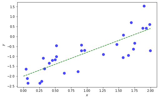
To test out our Gibbs sampler, let’s create some synthetic data and fit a model to it.

b0_true, b1_true, tau_true = -2, 1.2, 3

N = 30
x = np.random.uniform(0, 2, N)
y = b0_true + b1_true * x + np.random.normal(0, 1/np.sqrt(tau_true), N)

fig, ax = plt.subplots(1,1, figsize=(8,5))
xs = np.linspace(0,2,30)
ax.plot(xs, b0_true + b1_true*xs, 'g--')
ax.scatter(x, y, s=60, c='b', alpha=0.7)
ax.set(xlabel=r'$x$', ylabel=r'$y$')
plt.show()

Now we write a short loop to execute the Gibbs sampling algorithm:

def gibbs(x, y, n_runs, init, hyper):
    b0 = init['beta_0']
    b1 = init['beta_1']
    tau = init['tau']

    for _ in range(n_runs):
        b0 = sample_b0(x, y, b1, tau, hyper['mu_0'], hyper['tau_0'])
        b1 = sample_b1(x, y, b0, tau, hyper['mu_1'], hyper['tau_1'])
        tau = sample_tau(x, y, b0, b1, hyper['alpha'], hyper['beta'])
        yield (b0, b1, tau)

This will run n_runs times, at each iteration \(i\) yielding a triple of the parameter estimates \((\beta_0^{(i+1)}, \beta_1^{(i+1)}, \tau^{(i+1)})\).

Now we’ll set some initial values for the params, and set our 3 sets of hyperparameters, and run the sampler 1000 times.

# pick initial values for params
init = {'beta_0': 0, 'beta_1': 0, 'tau': 2}

# set hyperparameters
hyper = {'mu_0': 0, 'tau_0': 1,   # beta_0
         'mu_1': 0, 'tau_1': 1,   # beta_1
         'alpha': 2, 'beta': 1}   # tau
         
n_runs = 1000

# build trace
trace = [[b0, b1, tau] for b0,b1,tau in gibbs(x, y, n_runs, init, hyper)]
trace = np.array(trace)

fig, ax = plt.subplots(1,1, figsize=(10,4))
xs = np.arange(n_runs)
c = ['b', 'c', 'g']
labels = [r'$\beta_0$', r'$\beta_1$', r'$\tau$']
for i, true in enumerate([b0_true, b1_true, tau_true]):
    ax.plot(xs, trace[:,i], color=c[i], linestyle='-', alpha=0.8)
    ax.plot(xs, [true]*len(xs), color=c[i], linestyle='dotted', label=labels[i])
ax.legend(loc='upper center')
plt.show()

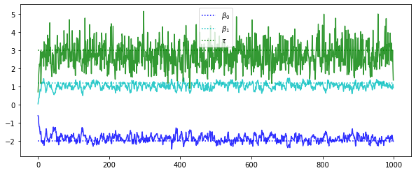
These traces are (kinda) hovering around the “true” values of the 3 parameters, with the most uncertainty in the noise parameter \(\tau\). Notice the first 50 or so iterations exhibit the “burn-in” as the sampler adjusts from its initialized values. In practice we typically discard a large portion of initial runs to ensure we’ve gotten past this burn-in.

Anyway, let’s visualize the (sampled) posteriors:

fig, axs = plt.subplots(1,3, figsize=(12,4))
for i, (ax, true) in enumerate(zip(axs.ravel(), [b0_true,b1_true,tau_true])):
    n, bins, patches = ax.hist(trace[100:,i], density=True, 
        facecolor=c[i], edgecolor='k', linewidth=0.5, alpha=0.5)
    patches[np.digitize(true, bins)-1].set_linewidth(1)
    patches[np.digitize(true, bins)-1].set_alpha(1)
    ax.plot([true]*2, [0,np.amax(n)], 'k--')
    ax.set(title=labels[i])
plt.show()

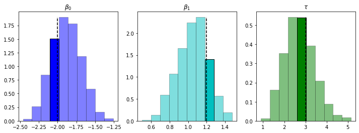
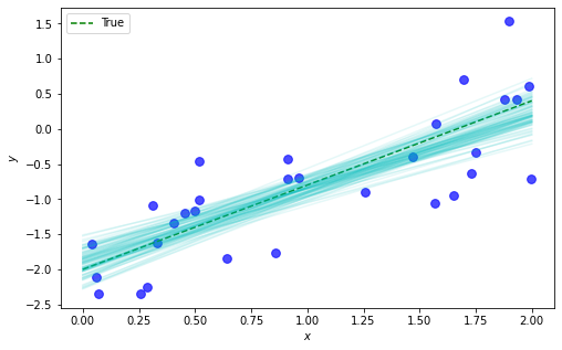
We’ve done an O.K. job capturing the true values (the dotted line in the highlighted bin), although not quite dead on. Having the full posteriors gives us the ability, similar to when we computed the full posterior directly, to quantify (and visualize) the uncertainty over possible estimators:

fig, ax = plt.subplots(1,1, figsize=(8,5))
ax.scatter(x, y, s=60, c='b', alpha=0.7)
xs = np.linspace(0,2,30)
ax.plot(xs, b0_true + b1_true*xs, 'g--', label='True')
for b0, b1 in trace[-100:,:2]:
    ax.plot(xs, b0 + b1*xs, 'c-', alpha=0.1)
ax.set(xlabel=r'$x$', ylabel=r'$y$')
plt.legend()
plt.show()

Next steps

A natural next step would be to explore Gibbs sampling on a more complex model – for example, linear regression with a higher input dimension (more covariates), larger hierarchical Bayes models, etc. We might also check out some of the pre-fab libraries for MCMC, like pymc3.

We could also explore variations on the vanilla Gibbs sampling we saw in this post, like blocking Gibbs sampling (to help break down the strong dependency between samples), collapsed Gibbs, or slice sampling. We could also take a step back and study the relation of Gibbs sampling to its parent, Metropolis-Hastings, or other Markov Chain Monte Carlo (MCMC) techniques.

(By the way, I love researching a new topic and finding all the wonderful blogs out there. I hope you’ve found this one useful!)