More linear regression -- getting Bayesian

This post is a follow-up to this post. My goal now is to explore basic ideas in the linear regression problem in a Bayesian setting — Bayesian linear regression. This post is really just a glorified note-to-self on key ideas and code recipes that I can reference later on, but maybe you will find it useful too.

But first, check out this sweet plot:

import matplotlib.pyplot as plt
import numpy as np
import scipy.stats

# hyperparams
alpha = 2   # prior precision
beta  = 25  # noise precision
s     = 0.1 # scale 
k     = 9   # number basis functions

# data
N = 30
ytrue = lambda xx: np.sin(2*np.pi*xx)
x = np.random.uniform(0,1, size=N)
y = ytrue(x) + np.random.normal(0, np.sqrt(1/beta), size=N)

# gaussian basis function
rbf = lambda x, mu: np.exp(-((x-mu)**2) / (2*s**2))
mus = np.linspace(0,1,k)  # 9 evenly spaced basis functions

# design matrix and plotting spaces
Xd = np.array([[rbf(xi, muj) for muj in mus] for xi in x])
xs = np.linspace(0,1,100)
Xs = np.array([[rbf(xi, muj) for muj in mus] for xi in xs])

# compute mean/cov of posterior predictive distribution
psig = np.linalg.inv(alpha * np.identity(k) + beta * np.dot(Xd.T, Xd))
pmu = beta * np.dot(np.dot(psig, Xd.T), y)
pvar = (1/beta) + np.dot(np.dot(Xs, psig), Xs.T)

fig, ax = plt.subplots(1,1, figsize=(10,5))

# plot true func and data
ax.plot(xs, ytrue(xs), 'c-')
ax.scatter(x, y, s=100, c='None', edgecolor='k')

# plot samples from posterior predictive
for _ in range(5):
    ys = np.random.multivariate_normal(np.dot(Xs, pmu), pvar)
    ax.plot(xs, ys, 'r-')

ax.set(xlim=[0,1], ylim=[-1.5,1.5], xlabel='$x$', ylabel='$y$')
ax.set_xticks([0,1])
ax.set_yticks([-2,2])
plt.show()

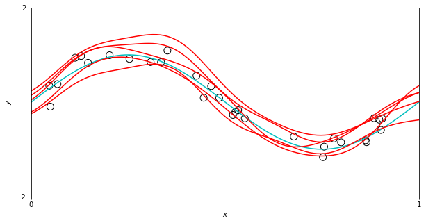
It appears we have a sinusoidal dataset, and we are showing several possible model fits to this data, from some class (or distribution) of very flexible models. This is in fact, basically what’s happening. This idea of “sampling possible models” is tied to the idea of a distribution over predictive outputs, and is fundamentally different than the point estimate approaches we saw in the last approach. Let’s dig into the math and make more cool looking plots.

Setup

Again, we begin with a dataset \(\mathcal{D} = \{(\xb_i, y_i)\}_N\), or \(\mathcal{D} = (X, \yb)\), with each input \(\xb_i \in\mathbb{R}^D\) and output or “target” \(y_i\in\mathbb{R}\).

We then decide to model this data with a linear model,

with additive, independent Gaussian noise

This yields a likelihood (“the likelihood of the data given our model”) of

To this point, we have only made choices on the type of model (linear) and type of noise (additive, iid, Gaussian). We have not made choices yet about how to make inference from the data of the parameters of our model, or make predictions for new data. In the previous post we examined several common approaches — “least squares,” maximum likelihood estimation, and regularized MLE (ridge regression). From a probabilistic perspective, however, these are not fully realized methods.

Computing the posterior (over the parameters)

Recall Bayes Rule, \(p(a\vert b) = p(b\vert a)p(a)/p(b)\). This rule follows from the axioms of probability, and is uncontroversial. What leads to differences of opinion, is when we apply this rule to the statistical learning problem at hand. Specifically, when we place the notion of a “prior” (that \(p(a)\) term) on our parameters.

From a “frequentist” perspective, this makes no sense — the parameter is a fixed (unknown) value, not a random variable. From a “Bayesian” perspective, since the parameter is unknown, we should model our uncertainty about it. In this paradigm, the rule is interpreted as:

In the previous post, we saw that if we consider a probabilistic but not fully Bayesian approach of just making a point estimate of the posterior, e.g. the MAP estimate, we recover other estimators (MLE, ridge regression) depending on our choice of prior. From a Bayesian perspective, this at least puts these methods on solid probabilistic footing — you’re not really computing an MLE estimator with an arbitrary penalty on the weights, you’re computing a MAP estimate with a Gaussian prior on the weights!

If we fully commit to this perspective, we should pursue computing the entire posterior (not a point estimate). And then, if we need to make predictions, we can employ our full knowledge of the parameters and the predictive posterior, into our prediction.

For a specific example, let’s specify a conjugate prior on \(\wb\), the zero-mean isotropic Gaussian:

This yields a posterior distribution \(p(\wb\vert \yb, X)\):

Note that the maximum (the mode), for a Gaussian, equals the mean \(\mb\), which you should recognize as the ridge regression estimate:

with \(\lambda = \alpha/\beta\) (the penalty term).

Example

Let’s show how the distribution over \(\wb\) changes as we update it with observations.

# reproduce Figure 3.7 from Bishop (p 155)
# note scipy "scale" = std dev, but cov = covariance

# hyperparams
alpha = 2  # prior precision
beta  = 25  # noise precision

# create data
N = 20
w_true = np.array([-0.3, 0.5])
X = np.ones((N,2))
X[:,1] = np.random.uniform(-1,1, size=N)
y = np.dot(X, w_true) + np.random.normal(0, np.sqrt(1/beta), size=N)

# spaces for plotting
wx, wy = np.mgrid[-1:1.1:.1, -1:1.1:.1]
z = np.dstack((wx, wy))
xs = np.linspace(-1,1,30)

fig, axs = plt.subplots(2,4, figsize=(14,6), sharey=True)

# col 0
# weight prior
rv = scipy.stats.multivariate_normal([0, 0], (1/alpha) * np.identity(2))
axs[0,0].contourf(wx, wy, rv.pdf(z), cmap='Blues')
for _ in range(6):
    s = rv.rvs()  # draw a random weight
    # axs[0,1].scatter(s[0], s[1], s=50, c='k', marker='+')
    axs[1,0].plot(xs, s[1]*xs + s[0], 'r-')

# cols 1-3
for j, n in enumerate([1,2,N]):
    Xt, yt = X[:n,:], y[:n]
    sig = np.linalg.inv(alpha * np.identity(2) + beta * np.dot(Xt.T, Xt))
    mu = beta * np.dot(np.dot(sig, Xt.T), yt)
    rv = scipy.stats.multivariate_normal(mu, sig)
    axs[0,j+1].contourf(wx, wy, rv.pdf(z), cmap='Blues')
    axs[1,j+1].scatter(Xt[:,1], yt, s=70, c='None', edgecolor='k')

    for _ in range(6):
        s = rv.rvs()
        axs[1,j+1].plot(xs, s[1]*xs + s[0], 'r-')

for ax in axs.ravel():
    ax.set(xlim=[-1,1], ylim=[-1,1])
    ax.set_xticks([-1,0,1])
    ax.set_yticks([-1,0,1])

for ax in axs[0,:].ravel():
    ax.set(xlabel=r'$w_0$', ylabel=r'$w_1$')
for ax in axs[1,:].ravel():
    ax.set(xlabel=r'$x$', ylabel=r'$y$')

plt.show()

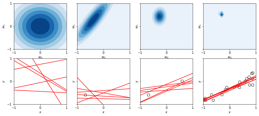
The first column depicts the zero-mean isotropic prior, and 6 lines that result from drawing 6 samples of \(\wb\) from this prior. In the second column, we introduce a single datapoint, and depict the resulting posterior over \(\wb\), now with positive correlation between \(w_0\) and \(w_1\) – this makes sense because the larger we make the intercept (\(w_0\)), the steeper we need to make the slope (\(w_1\)) to still catch the datapoint, and since the data point is left of the \(y\)-axis, the two parameters will change in the same direction. In the third column, two datapoints significantly sharpen our prior (which follows since you only need 2 points for a line), even further sharpened in the last column.

Posterior predictive

We usually aren’t interested in admiring the value of \(\wb\), but instead, making predictions of \(y\) for new values of \(\xb\). In the frequentist paradigm, we’d use a point estimate of \(\wb\) (e.g. MLE) in our linear model \(f(\xb) = \xb^T \wb\). But now, we have an entire distribution over \(\wb\), capturing all our uncertainty and knowledge based on observation of data — why not use all of it?

So, under the Bayesian perspective, evaluate the predictive distribution (or posterior predictive),

Recall \(p(t\vert X,\wb) = \mathcal{N}(\xb^T\wb, \beta^{-1})\) and the posterior weight distribution \(p(\wb\vert \yb,X)\) is given above. With some effort, we can convolve these two distributions, giving

Here, \(\mb\) and \(\Sigma\) are the mean and covariance of the posterior weight distribution. It feels easily intuitive that the mean of the predictive distribution should be just \(\mb^T \xb\). The variance \(\sigma^2\) also has a nice interpretation: it is the noise from the data (\(1/\beta\)) and the uncertainty associated with \(\wb\) encoded in \(\Sigma\). As we get more data, the contribution from \(\Sigma\) goes to zero and our only variance comes from the noisiness of the data.

Example

Let’s test this out on some sinusoidal data with additive white noise, and employing the Gaussian basis function

with \(\mu_j\) evenly spaced across the domain.

# example from Bishop Figure 3.8 (p 157)

# hyperparams
alpha = 2   # prior precision
beta  = 25  # noise precision
s     = 0.1 # scale 
k     = 9   # number basis functions

# data
N = 25
ytrue = lambda xx: np.sin(2*np.pi*xx)
x = np.random.uniform(0,1, size=N)
y = ytrue(x) + np.random.normal(0, np.sqrt(1/beta), size=N)

# gaussian basis function
rbf = lambda x, mu: np.exp(-((x-mu)**2) / (2*s**2))
mus = np.linspace(0,1,k)  # 9 evenly spaced basis functions

# design matrix
Xd = np.array([[rbf(xi, muj) for muj in mus] for xi in x])

# for plotting
xs = np.linspace(0,1,100)
Xs = np.array([[rbf(xi, muj) for muj in mus] for xi in xs])


fig, axs = plt.subplots(2,2, figsize=(12,10), sharex=True, sharey=True)

# 0,0 plot prior
# weight prior
rv = scipy.stats.multivariate_normal(np.zeros(k), (1/alpha) * np.identity(k))
for _ in range(5):
    ws = rv.rvs()  # sample a weight from prior
    axs[0,0].plot(xs, ytrue(xs), 'c-')
    axs[0,0].plot(xs, np.dot(Xs, ws), 'r-')

# 0,1 - 1,0 - 1,1
for ax, n in zip([axs[0,1], axs[1,0], axs[1,1]], [2, 4, N]):
    Xt, yt = Xd[:n,:], y[:n]
    psig = np.linalg.inv(alpha * np.identity(k) + beta * np.dot(Xt.T, Xt))
    pmu = beta * np.dot(np.dot(psig, Xt.T), yt)
    pvar = (1/beta) + np.dot(np.dot(Xs, psig), Xs.T)
    
    # plot true func and data
    ax.plot(xs, ytrue(xs), 'c-')
    ax.scatter(x[:n], y[:n], s=80, c='None', edgecolor='k')
    
    # plot samples from posterior predictive
    for _ in range(5):
        ys = np.random.multivariate_normal(np.dot(Xs, pmu), pvar)
        ax.plot(xs, ys, 'r-')

for ax in axs.ravel():
    ax.set(xlim=[0,1], ylim=[-1.5,1.5], xlabel='$x$', ylabel='$y$')
    ax.set_xticks([0,1])
    ax.set_yticks([-1.5,1.5])

plt.tight_layout()
plt.show()

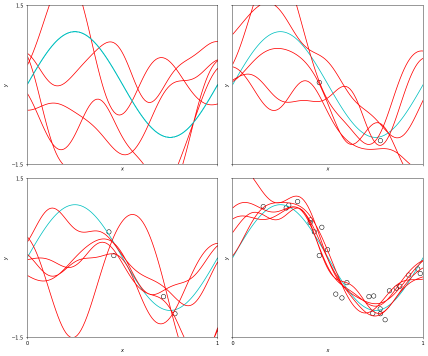
These function samples give a sense of the variance of the predictive distribution, and we could actually plot this variance spread, although I didn’t because the plot was pretty busy as-is.

Other topics

• Kernel methods. Through a bit of algebra (the “kernel trick”), you can rewrite the predictive posterior model \(y(\xb) = \mb_T \phi (\xb)\) as \(y(\xb) = \sum_i k(\xb, \xb_i)y_i\), where \(k(\xb,\xb')=\beta \phi(\xb)^T \Sigma \phi(\xb')\) is the “equivalent kernel.” We can similarly rewrite the covariance. This observation allows us to work just with kernels, and discard working with basis functions entirely. In this way, we can broaden our model, which leads to the framework of Gaussian processes. We can broaden many standard models by introducing kernel methods.

• Empirical Bayes. We assumed \(\alpha\) and \(\beta\) (the parameters governing the variance of the weight prior and additive noise) had known values, which we substituted directly. To be more fully Bayesian, we should simply place a prior distribution over these parameters. Unfortunately, the computation of the predictive posterior becomes intractable regardless of our choice of prior. One compromise is to integrate over just \(\wb\) and then maximize the resulting marginal likelihood function – this is called empirical Bayes or the evidence approximation.

• Fully Bayes. To go all the way, and place priors on all parameters, we need to introduce approximate inference. In variational inference, we use an analytically tractable approximation to the posterior. In Markov chain Monte Carlo methods, we use sampling techniques to approximate the distribution.

Lots more to learn about. Thanks for reading!