Linear Regression (again)

Linear regression is a workhorse, and its exposition has been done to death in every textbook and blog and lecture note on the planet. However, I find there are certain sticking points I encounter every time I have to re-learn portions of this subject, that I find clarified in differnt texts but never all in one place. So the purpose of this post is to give the exposition as I would want, for future me, re-learning this stuff.

If you’re not me, let me just introduce this subject by saying the introductory treatment of linear regression as a “least squares” model is very plain — but the waters run much deeper. Deriving linear regression probabilistically, we encounter many known and new flavors, culminating with a fully Bayesian treatment, and with connections to PCA, regularization, and other concepts along the way.

Preliminaries

We begin with a dataset \(\mathcal{D} = \{(\xb_i, y_i)\}_N\), or \(\mathcal{D} = (X, \yb)\), with each input \(\xb_i \in\mathbb{R}^D\) and output or “target” \(y_i\in\mathbb{R}\).

We then decide to model this data with a linear model,

where \(\varepsilon\) represents some error between our model and reality.

An intro to linear regression typically begins with “ordinary least squares”, where we choose weights \(\wb\) that minimize the (mean) squared error \((y_i - \xb_i^T \wb)^2\) over all data,

Let’s visualize this with a little toy example.

import matplotlib.pyplot as plt
import numpy as np

# data
N = 20
w1_true = 1.5
x = np.linspace(0, 1, N)
y = w1_true * x + np.random.normal(0, 0.3, size=N)

# plot
fig, ax = plt.subplots(1,1, figsize=(9,5))

# draw data
xs = np.linspace(0,1, 30)
ax.scatter(x, y, c='b', s=70, alpha=0.7)
ax.plot(xs, w1_true * xs, 'c--', label='True')

# draw model
w0_est, w1_est = 0.1, 1.3
ax.plot(xs, w1_est * xs + w0_est, 'k-', label='Model')
for xi,yi in zip(x,y):
    ax.plot([xi,xi], [w1_est * xi + w0_est, yi], 'b-', alpha=0.5)

ax.set(xlabel=r'$x$', ylabel=r'$y$')
plt.show()

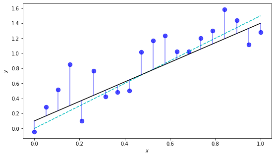
This example doesn’t actually depict the \(\wb_{\text{OLS}}\), just a decent-looking model. To find \(\wb_{\text{OLS}}\), we need to find the minimum of the objective function before. We’ll save this for later.

We can apply a basis transformation \(\mathbf{\phi}:\mathbb{R}^D \rightarrow \mathbb{R}^{K+1}\) to the \(\xb\), for example a polynomial expansion \(\mathbf{\phi}_k(x) = (x^k, x^{k-1}, ..., x, 1)\). Under this expansion, the \(N\times D\) data matrix \(X\) transforms to the \(N\times (K+1)\) “design matrix” \(\Phi\). This doesn’t change any of the math, so we’ll just work with \(\xb\) for now.

Thinking probabilistically

We should wonder — why squared error, and not absolute value? why a linear model? what about outliers? what is the meaning of life? Etc. Introducing a probabilistic foundation will reveal a greater depth to this model.

First, assume the additive noise (\(\varepsilon\)) is distributed as

Therefore, each \(y_i \sim \mathcal{N}(\xb_i^T \wb, \sigma^2)\), and since the noise is iid,

This is the “likelihood”. More generally \(p(\mathcal{D}\vert \mathbf{\theta})\), the likelihood of the data given the parameters – in this case, we have chosen not to model any distribution over the \(\xb\) (inputs), and we’ve specified a model with specific parameters.

MLE

Then we decide to estimate the parameters \(\wb\) under this structure. A probabilistically minded approach might be to choose parameters which maximize the likelihood they led to the data we observe – this is maximum likelihood estimation (MLE).

Note we’re actually maximizing the log-likelihood, which we’re allowed to do because the log is a uniform transformation (and we’re just seeking the argmax), and which we want to do because it will make the math easier.

Here’s the nifty part: our likelihood is iid Gaussians with mean \(\xb_i^T \wb\), so when we take a log we turn the product into a sum, cancel out the exponentials, and get a sum over that exponent from a normal distribution. Which reminds us of the sum-of-squares form. Let’s make this explicit.

Define the log-likelihood as a function \(\ell\), and note for our linear model,

When we go to maximize \(\ell(\wb)\), or minimize \(-\ell(\wb)\), we can ignore the constants, and just have

which is also, of note, identical to the “least squares” estimator! I love this.

We can actually solve this explicitly. Writing in matrix form,

The gradient is \(\nabla \big(-\ell(\wb)\big) = X^TX\wb - X^T\yb\), which we set to zero and get

Geometric interpretation

This carries a nice geometric interpretation: imagine \(X\) as a \(D\)-dimension linear subspace living in \(\mathbb{R}^N\), and \(\yb\) as a vector in \(\mathbb{R}^N\) – note, each column vector \(\tilde{\xb}_j\) of \(X\) is an \(N\) dimensional vector which lies in \(\mathbb{R}^N\), not row vectors which are datapoints. Then imagine \(\hat{\yb}\) is the projection of \(\yb\) onto \(X\) (that minimizes the L2 distance).

We know \(\hat{\yb}\in\text{span}(X)\), so it must equal some linear combination of (column) vectors, i.e., \(X\wb\). The residual/distance vector \(\yb-\hat{\yb}\) which is minimal is orthogonal to \(X\) (orthogonal to every column vector of \(X\)), i.e. \(\tilde{\xb}_j^T (\yb-\hat{\yb}) = 0\) for all \(j\). That is, \(X^T(\yb-X\wb) = 0\), which leads to the same system of equations as above.

Example

Let’s create a well-behaved, but slightly tricky dataset of sinusoidal data with Gaussian noise. We’ll then fit a straight linear model and try some basis expansions with different degrees of polynomial.

# sinusoidal data with Gaussian noise
N = 20
x = np.linspace(0, 2*np.pi, N)
y = np.sin(x) + np.random.normal(0, 0.5, size=N)

# basis expansion
phi = lambda xi, k: [xi**ki for ki in range(k+1)]

# plot
fig, ax = plt.subplots(1,1, figsize=(9,5))

xs = np.linspace(0, 2*np.pi, 100)
ax.plot(xs, np.sin(xs), 'g--', alpha=0.5, label='Actual')
ax.scatter(x, y, s=70, c='b', alpha=0.5)

for k, c in zip([1, 3, 10], ['k', 'b', 'c']):    
    # create design matrix (inefficient but readable)
    X = np.array([phi(xi, k) for xi in x])
    Xs = np.array([phi(xi, k) for xi in xs]) # for plot only
    
    # compute w_MLE
    w = np.linalg.inv(np.dot(X.T, X))
    w = np.dot(np.dot(w, X.T), y)
    ax.plot(xs, np.dot(Xs, w), color=c, linewidth=2, label=f'$k={k}$')
    
ax.legend()
ax.set(xlabel=r'$x$', ylabel=r'$y$')
plt.show()

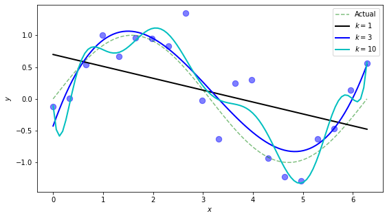
This is cool. We see the straight line does its best but doesn’t have the flexibility to provide a worthwhile model of the data. The degree-3 polynomial seems, qualitatively, to do a good job approximating the true function (sine) generating the data. The degree-10 polynomial is overfitting quite a bit, and we would expect it to do poorly if we began testing it on new data.

Let’s take a look at the likelihood function. We’ll use a linear model (or equivalently \(k=1\)) so \(\wb\) is a 2-dimensional vector and we can visualize both its components in a 2-d plot. (This does require us to create a grid of (w0,w1)’s to plot, which is a PITA.)

# instead of using phi(x, 1), we'll just manually add the column of ones for the intercept w_0
X = np.ones((N,2))
X[:,1] = x

# compute actual w_MLE (optimum)
w = np.linalg.inv(np.dot(X.T, X))
w = np.dot(np.dot(w, X.T), y)

# we need a grid of w's (w0, w1)
w0, w1 = (-.5,1.5), (-1,1)
m  = 64  # number partitions in grid
w0g, w1g = np.linspace(w0[0], w0[1], m), np.linspace(w1[0], w1[1], m)

# convert to grid, Xm and Ym both shape=(m,m)
# each row of W0m is w0g, each col of W1m is w1g
W0m, W1m = np.meshgrid(w0g, w1g)

# convert to list with shape=(m^2,2)
# lists every point in the grid, from bottom left to top right
W = np.array([W0m.ravel(), W1m.ravel()]).T

# recall ell = 0.5 (y-Xw)^T (y-Xw)
# using a loop is very hacky, but easier to read than matrix maneuvers
ells = []
for wx in W:
    t = y - np.dot(X, wx)
    ells.append(0.5 * np.dot(t.T, t))
ells = np.array(ells).reshape((m,m))

fig, ax = plt.subplots(1,1, figsize=(9,7))
levels = np.linspace(0,240,20)
cb = ax.contourf(W0m, W1m, ells, cmap='Blues', levels=levels)
ax.contour(W0m, W1m, ells, colors='k', levels=levels, linewidths=0.5)
ax.scatter(w[0], w[1], c='k', marker='o')
ax.set(xlabel=r'$w_0$', ylabel=r'$w_1$')
plt.colorbar(cb)
plt.show()

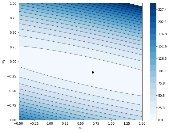
Notice:

• there appears to be a unique optimum (minimum). This matches what we can show mathematically, that the objective function is convex.
• the optimum is very flat. Because the linear model doesn’t fit the data very well, it doesn’t matter much what intercept (\(w_0\)) you pick. I bet if we took the noise out of the data, the best model might be \(\wb = (0,0)\), i.e. no model at all.
• if we were solving for this optimum numerically, the flat optimum would cause convergence issues, but that’s a completely different post.

A dusting of Bayes

Applying Bayes rule to this situation, we have

(Note: the denominator has a few different names — model evidence, marginal likelihood, prior predictive density – and you’ll note by Bayes rule it should be \(p(X, \yb)\) but we’ve left \(\yb\) conditional \(X\). This requires justification but is standard under the assumption \(X\) is chosen/designed/controlled and therefore not a variable part of the data.)

This Bayesian formulation makes explicit the paradigm there is uncertainty in the parameters, \(\wb\), and we can only hope to define a distribution over them. Specifically, we should first identify our prior belief about the parameters (\(p(\wb)\)) and then update that prior with evidence (the data) to derive the posterior (\(p(\wb\vert \yb,X)\)).

But maybe that’s too hard, or overkill, or we don’t wanna, so we just make a point estimate of the posterior — for example, the maximum aposteriori (MAP) estimate, which gives the mode (the max) of the posterior.

The MAP estimate, in general, and taking logs, is:

where notice the unruly denominator of Bayes rule disappears since it’s constant in \(\wb\).

Reinterpreting the MLE estimator. Another way to interpret \(\hat{\wb}_{\text{MLE}}\) is as a MAP estimate with a uniform prior on \(\wb\). (A uniform prior will appear as a constant in the objective function above, and disappear.)

With this all in mind, some natural next avenues to explore:

• change the Gaussian assumption on error (e.g. using the Laplacian, “robust linear regression”)
• change the prior (e.g. using a Gaussian, which leads to ridge regression, or a Laplacian, which leads to the LASSO)
• compute the entire posterior (which leads to Bayesian linear regression)

Ridge regression

We may want to use a more complex model (like a polynomial basis expansion), but are concerned the model will “overfit,” like the degree-10 polynomial did earlier. We can encourage the parameters to be small by imposing a zero-mean Gaussian prior on the \(\wb\),

Using the MAP estimate, and following a similar derivation from above, leads to the objective function

where we often define \(\lambda = \sigma^2/\tau^2\). Intuitively, the size of the weight vector \(\wb\) now acts as a penalty term on the objective function, and choosing a higher value for \(\lambda\) will increase the penalty.

This also yields an explicit solution,

Although I always thought the augmentation of the \(X^T X\) matrix by a diagonal ridge of \(\lambda\)’s is what gives the estimator its name, this is (according to the internet) not true. It refers to the flat ridge of the objective function (the likelihood) that results from multicollinearity — ridge regression fixes the “ridge”.

Example

# hyperparams
k = 6  # degree of polynomial
# lambda also a hyperparam, will test in plot

# sinusoidal data with Gaussian noise
N = 20
x = np.linspace(0, 2*np.pi, N)
y = np.sin(x) + np.random.normal(0, 0.5, size=N)

# create design matrix (inefficient but readable)
phi = lambda xi: [xi**ki for ki in range(k+1)]
X = np.array([phi(xi) for xi in x])

# create data for plot
xs = np.linspace(0, 2*np.pi, 100)
Xs = np.array([phi(xi) for xi in xs])

# plot
fig = plt.figure(figsize=(14,6))
gs = fig.add_gridspec(2, 2, width_ratios=[3, 1.5])
ax1 = fig.add_subplot(gs[:,0])   # scatter
ax2 = fig.add_subplot(gs[0,1])  # bar chart top
ax3 = fig.add_subplot(gs[1,1])  # bar chart bottom

ax1.plot(xs, np.sin(xs), 'g--', alpha=0.5, label='Actual')
ax1.scatter(x, y, s=70, c='b', alpha=0.5)

for lam, c, ax in zip([0, 10], ['c', 'k'], [ax2, ax3]):
    # compute w_ridge
    w = np.linalg.inv(lam * np.identity(k+1) + np.dot(X.T, X))
    w = np.dot(np.dot(w, X.T), y)
    ax1.plot(xs, np.dot(Xs, w), color=c, linewidth=2, label=f'$\\lambda={lam}$')
    ax.bar(range(len(w)), w)
    ax.text(k-2, np.amax(w)*.9, f'$\\lambda={lam}$')
    ax.set_xticks(range(k+1))
    ax.set_xticklabels([f'$w_{i}$' for i in range(k+1)])
   
ax1.legend()
ax1.set(xlabel=r'$x$', ylabel=r'$y$')
plt.show()

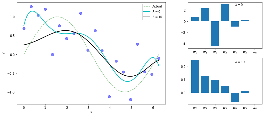
We know a high degree polynomial will overfit this dataset. Here, we see a degree-6 polynomial overfitting when \(\lambda=0\) (i.e. ordinary regression), but using ridge regression with a high penalty term of \(\lambda=10\), we get what appears to be a more sensible model. Also notice the weights are smaller and more balanced, we don’t have large competing terms canceling each other out.

Next steps

So far we reintroduced the basic ideas of linear regression from a probabilistic perspective, including the context of the Bayesian approach, culminating with a view of ridge regression as a MAP estimate of the posterior with a zero-mean Gaussian prior.

We’d like now to take a fully Bayesian approach to linear regression. That is, instead of taking a MAP estimate, let’s compute the entire posterior. And instead of using a point estimate of the parameters to make predictions, let’s use the “predictive posterior” which takes into account our uncertainty over the parameters. And instead of arbitrarily choosing values for hyperparameters (like the variance of the prior), we should attempt to find ways to infer those from the data.