Gaussian Processes - how do they work again?

Gaussian processes are a workhorse in machine learning, and connect many core ideas – kernels, Bayesian approaches to supervised learning, stochastic processes. For me though, GPs felt very weird at first, and it was tough to grok what was going on, much less wade through the gnarly derivations.

My goal is to explain this how I’d want it explained to me. So, I assume you’re me – some background in probability, familiarity with foundational machine learning concepts, basic coding proficiency, and a fleeting attention span that demands non-rigorous explanations the first go-around.

So I’m going to skip things like re-deriving Gaussian distribution properties, or linear regression in a Bayesian context. I assume you’ve seen this before, or are comfortable looking it up. (I can’t rederive the predictive posterior for a Bayesian linear regression off the cuff, but I don’t particularly want to slog through it again right now either.)

My favorite references for this are the gorgeous, interactive Distill.pub article (btw, Distill.pub RIP, so sad), the resources on gaussianprocess.org including this slick interactive, this friendly orientation that is maybe closest to the tone I’m aiming for, Peter Roelant’s blog on GPs (his blog is really good, check it out).

And of course, the standard text by Rasmussen and Williams.

Introductions

My first introduction to Gaussian processes was probably with a beautiful picture like this:

(Source)

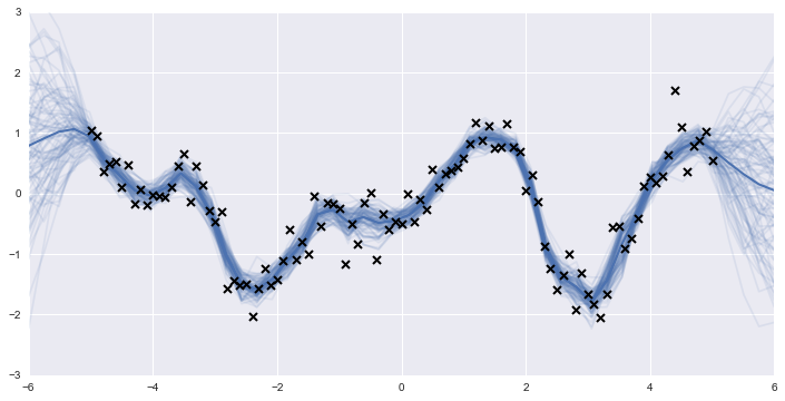
and a really enticing, intuitive explanation that a GP was a distribution over possible functions, and here we have applied the Bayesian approach of conditioning on training data, to get a predictive posterior distribution of functions that incorporated that information.

I could imagine the smooth little functions being sampled all over the space, then training data conditioning out a bunch of them, etc.

Sold.

But I found it tough to grasp how the mechanics of it worked. Definitions like “A Gaussian process is a collection of random variables, any finite number of which have a joint Gaussian distribution” just made me think, um, ok?

Mini-GP

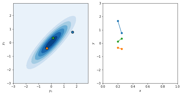
As a thought experiment, consider a bivariate Gaussian random variable, dimension \(m=2\), with zero mean, and covariance defined in terms of some set \(X\) of vectors \(\mathbf{x}\in\mathbb{R}^d\) (and if you like, imagine \(d=1\) for now). Make \(\vert X\vert = 2\).

Specifically, let \(K\) be a function that magically transforms the \(\mathbf{x}\)’s into a valid covariance matrix of dimension \(2\times 2\).

We could also think of this setup in terms of a function: input \(x\), output (random) \(y\), denoted \(f(\mathbf{x})\).

Let’s further say that our \(K\) is constructed so that, the closer \(\mathbf{x}_1\) and \(\mathbf{x}_2\) are together, the higher the correlation of \(y_1\) and \(y_2\). It would help me at this point to have a concrete example of such a function.

One way to do that is to define the covariance of \(f(\mathbf{x})\) and \(f(\mathbf{x}')\), that is the entry \(K_{x,x'}\) of \(K\), with the covariance function,

This is called the squared exponential or radial basis function (RBF). You can see, as \(\mathbf{x}\) and \(\mathbf{x}'\) get closer (the norm of their difference grows smaller), the function (i.e. the covariance) approaches 1.

Why this works, why the RBF is a common choice, and why we know this kernel function creates a positive semi-definite covariance matrix, let’s worry about later. But this is nice: with closer inputs (x’s), we get closer outputs (y’s).

Let’s test it out. We’ll setup the bivariate Gaussian for two \(x\) inputs that are fairly close to each other, and take a few samples. Then, in keeping with the mindset that this creates a function, we’ll plot the samples against the inputs.

# this computes the covariance matrix with an RBF kernel
# scipy's distance_matrix can handle different size matrices
# X -> (m,k), X_ -> (n,k), returns -> (m,n)
def rbf(X, X_, ls=1):
    # this handles if X or X_ are lists of 1d
    X = X.reshape((-1,1)) if len(X.shape) == 1 else X
    X_ = X_.reshape((-1,1)) if len(X_.shape) == 1 else X_

    # compute rbf and return
    return np.exp(-(1/(2*ls)) * np.power(distance_matrix(X, X_), 2))

# create a bivariate gaussian dist instance
xs = np.array([0.2, 0.25])  # as this get closer, correlation will increase
K = rbf(xs, xs, ls=0.01)
rv = scipy.stats.multivariate_normal([0, 0], K)

# generate data to plot a clean bivariate gaussian
x, y = np.mgrid[-3:3:.1, -3:3:.1]
data = np.dstack((x, y))
z = rv.pdf(data)

# plot
fig, axs = plt.subplots(1,2, figsize=(10,5))

# plot bivariate gaussian
axs[0].contourf(x, y, z, cmap='Blues')

# plot a few sample y's from input x's
for _ in range(3):
    ys = np.random.multivariate_normal([0,0], K)
    axs[0].scatter(ys[0], ys[1], s=70, marker='o', edgecolors='k')
    axs[1].plot(xs, ys, marker='o', linestyle='-')
axs[1].set(xlim=[0,1], ylim=[-3,3])
axs[0].set(xlabel=r'$y_1$', ylabel=r'$y_2$')
axs[1].set(xlabel=r'$x$', ylabel=r'$y$')

If I had more time, we could code this up as an interactive plot, kinda like what they do on this infinitecuriosity.org site, but maybe not quite so insanely well-done and complex.

Another thing we’d want to do is increase the dimension \(m\) of the Gaussian (that is, the number of inputs). That’s what they do, more explicitly, in this post, and what we’ll do in the next section.

Function space view expanded

Our approach so far has been to understand a Gaussian process through a “function space view” – i.e. viewing the process as a distribution in function space.

Let’s build that out now. First, a pedantic pause: to me, it’s at first tricky to keep straight that the vectors of the set \(X\) are dimension \(d\), and the dimension of the Gaussian we’re sampling from is the size of the set \(X\), \(m\). Keeping that in mind, we can grow this idea beyond \(m=2\). Just keep growing the size of \(X\) — 100 inputs, 1000 inputs, etc. The Gaussian can grow indefinitely because it is completely characterized by the covariance function \(k\)! And we know that the \(y_i\) corresponding to \(x_i\) will be close to its \(y\) neighbors only if \(x_i\) is close to its \(x\) neighbors, so we can rest assured that all these new inputs will create corresponding \(y\)’s that make a smooth, curvy looking function.

This gives us the informal impression the function \(f\) will look, and be, continuous.

Put another way, the Gaussian process is a distribution over functions from \(\mathbb{R}^d\) to \(\mathbb{R}\), characterized by the kernel \(k(\cdot, \cdot)\). To sample from the process (the distribution), we input a finite subset \(X_*\), resulting in \(f_*\).

Let’s try with a bigger input set. We’ll plot several function samples from the same, evenly distributed input set. The first sample we’ll show the discrete points, which is really all we know. The other samples we’ll fudge and interpolate a curve.

m  = 50   # number of inputs
ls = 0.01  # length-scale of RBF

xs = np.linspace(0,1,m)
K = rbf(xs, xs, ls=ls)

fig, ax = plt.subplots(1,1, figsize=(9,5))
fs = np.random.multivariate_normal(np.zeros(m), K)
ax.scatter(xs, fs, s=10, alpha=0.7)
for i in range(4):
    fs = np.random.multivariate_normal(np.zeros(m), K)
    ax.plot(xs, fs, linewidth=2, alpha=0.7)
ax.set(xlabel=r'$x$', ylabel=r'$y$')

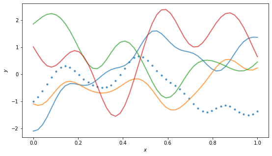
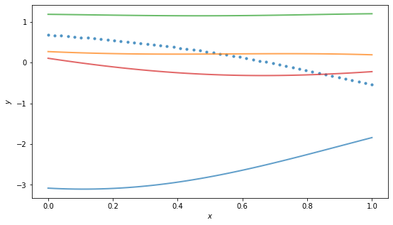
By the way, for the RBF kernel, the (hyper)parameter \(\ell\) is called the “length scale” and roughly controls the distance you have to move in input space for a significant change in function output. Above example has \(\ell = 0.01\), so it doesn’t take much change in \(x\) to get changes in \(y\), and the function is quite wiggly. Using a larger scale, say \(\ell=1\), we get “flatter” functions:

Incorporating data

So far we’ve just been getting familiar with the mechanics of sampling functions from this distribution. Roughly, we fix the inputs \(X\), and that defines a distribution of outputs \(Y\) that, through the magic of the kernel, create a continuous function.

We’ll now place this in a Bayesian, machine learning context.

Let the distribution as-is represent a prior over possible functions describing our data, but with no knowledge of the data. So far we’ve just been drawing samples from this prior. Once we observe data, we will compute the posterior distribution of functions, and be able to make predictions.

Let’s refer to our “training data” as \(X\), and our “test data” as \(X_*\). Training data will be a small little set of pairs \((\mathbf{x}_i, y_i)\). “Test” data will then be whatever size sample we want to look at, probably a lot, like before (and dictate the dimension \(m\) of our distribution).

One way to accomplish this is to consider first the joint distribution formed from training and test data:

where we note \(\mathbf{f}\) is fixed.

To extract the posterior distribution over \(\mathbf{f_*}\) conditioned on everything we know, we condition the joint distribution on the observations and get (through a good bit of algebraic maneuvers):

We’ll see this form again later. For now, let’s try it out with some made-up data:

n = 100   # number of inputs
ls = 0.05 # length-scale

# training data
x = np.array([0.2, 0.45, 0.8])
f = np.array([1, 0.1, -0.5])

# "test" data
xs = np.linspace(0,1,n)

Kxx = rbf(x, x, ls=ls)
invKxx = np.linalg.inv(Kxx)
Kx_ = rbf(x, xs, ls=ls)
K_x = rbf(xs, x, ls=ls)
K__ = rbf(xs, xs, ls=ls)

mean = np.dot(np.dot(K_x, invKxx), f)
covar = K__ - np.dot(np.dot(K_x, invKxx), Kx_)

fig, ax = plt.subplots(1,1, figsize=(8,5))

# plot function samples
for _ in range(5):
    fsc = np.random.multivariate_normal(mean, covar)
    ax.plot(xs, fsc, alpha=0.7)

# plot data
ax.scatter(x, f, s=20, c='k')

# plot 2*std
std = np.sqrt(np.diag(covar))
ax.fill_between(xs, mean + 2*std, mean - 2*std,
                facecolor='b', alpha=0.1)

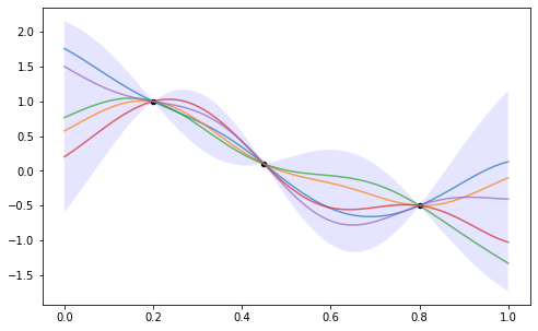
Beautiful. We implicitly made an assumption that the data was noise-free – we can loosen this assumption, and the posterior doesn’t pass tightly through the data. Let’s boot that topic to another time.

Weight space view

It feels a little wobbly how we come to this magic “kernel” function. Why is it what it is? What does it signify? Can we just make up whatever functions we want?

To shed light on this, we should re-develop the Gaussian process from the “weight space view.”

Recall the standard linear regression model, \(f(\mathbf{x}) = \mathbf{x}^T \mathbf{w}\), which we may make more flexible by transforming the inputs,

for some basis transformation \(\mathbf{\phi}(\cdot) \ : \ \mathbb{R}^D \rightarrow \mathbb{R}^N\). We refer to \(\mathbb{R}^N\) as “feature space”.

The posterior predictive distribution (using a Bayesian linear regression approach, derivation omitted, see Rasmussen) is then:

with \(\Phi = \Phi(X)\) the aggregation of all \(\phi(x)\), and \(A = \sigma_n^{-2}\Phi\Phi^T + \Sigma_p^{-1}\).

So to compute this, we need to invert \(A\), which is \(N\times N\). That’s a little rough. So, with a little algebra work, we can instead rewrite this in such a way that the feature space always appears in the form \(k(x,x') = \phi(x)^T \Sigma_p \phi(x')\). This function \(k(x,x')\) we call the kernel. For a single point, we can rewrite the above as,

And now, note that this predictive posterior, rewritten in terms of the kernel, if we expanded back out to the entire training set, is exactly what we had previously from the function space view.

The benefit now, is that we see the meaning of the kernel. When we use some \(\mathbf{\phi}\) to transform the input space from \(\mathbb{R}^d\) to \(\mathbb{R}^n\), the algebra simplifies to a new function, the kernel. So in fact, we often don’t need to fret about choosing the right transformation – we can just work with kernels, and, for example, choose one that corresponds to an infinite basis expansion, and then just fret about regularizing the model sufficiently instead.

This is a common pattern that arises in many other machine learning contexts, not just GPs, and relates to deep concepts like the representer theorem that I don’t grasp yet.

Expanding the input space

Anyway, let’s close with more pictures. We’ve so far limited the input space to 1-dimension, but we can easily expand. The hardest part is adapting our code to accommodate the changes, but the math is quite the same.

Here we sample from a prior in 2-dimensions. (Note we’ve improved our code for computing \(K\) to take advantage the scipy function pdist which computes pairwise distances.)

# params
x1, y1 = 10, 10
m  = 30  # number partitions in grid
ls = 2   # length scale of GP

# create grid coords
xg, yg = np.linspace(0, x1, m), np.linspace(0, y1, m)

# convert to grid, Xm and Ym both shape=(m,m)
# each row of Xm is xg, each col of Ym is yg
# so the (x,y) coords in the (1,2) grid square
# are (xg[1], yg[2]) or (Xm[2,1], Ym[2,1])
Xm, Ym = np.meshgrid(xg, yg)

# convert to list with shape=(m^2,2)
# lists every point in the grid, from bottom left to top right
X = np.array([Xm.ravel(), Ym.ravel()]).T

# centered on grid square
X += (x1 / m) / 2

# draw sample from GP
K = rbf(X, X)
Y = np.random.multivariate_normal(np.zeros(len(X)), K)

And now we have our sample \(Y\) as before, still a list of scalars, each \(y_i\in\mathbb{R}\). Let’s plot:

fig, ax = plt.subplots(1,1, figsize=(10,8))

# set level surface splits to display. 15 seems like a good amount
levels = np.linspace(0,np.amax(Y),15)

# display contour lines
ax.contour(Xm, Ym, Y.reshape(m,m), colors='k', levels=levels, linewidths=1)

# display contour fill
cs = ax.contourf(Xm, Ym, Y.reshape(m,m), cmap='Blues', levels=levels)

plt.colorbar(cs)

Ahh yeah. Doesn’t it evoke topo maps, weather patterns, … well, in fact, an early use case of GPs was in geostatistics, where it is known as kriging (named after Danie Krige, a South African guy who wrote a master’s thesis about it in the ’50s, which is kinda cool), and typically with 2D inputs corresponding to physical spaces.

Let’s try fitting to some data.

# params
x1, y1 = 10, 10
m  = 30  # number partitions in grid
ls = 1   # length scale of GP

# training data
x = np.array([ [2,4], [2.5,5], [8,7] ])
f = np.array([ 5, 3, -4 ])

# create grid coords ("test data")
xg, yg = np.linspace(0, x1, m), np.linspace(0, y1, m)
Xm, Ym = np.meshgrid(xg, yg)
Xs = np.array([Xm.ravel(), Ym.ravel()]).T
Xs += (x1 / m) / 2

Kxx = rbf(x, x, ls=ls)
invKxx = np.linalg.inv(Kxx)
Kx_ = rbf(x, Xs, ls=ls)
K_x = rbf(Xs, x, ls=ls)
K__ = rbf(Xs, Xs, ls=ls)

mean = np.dot(np.dot(K_x, invKxx), f)
covar = K__ - np.dot(np.dot(K_x, invKxx), Kx_)

and let’s look at the contour plot again:

fig, ax = plt.subplots(1,1, figsize=(10,8))

# sample function from GP
Y = np.random.multivariate_normal(mean, covar)

# plot
levels = np.linspace(np.amin(Y),np.amax(Y),15)
ax.contour(Xm, Ym, Y.reshape(m,m), colors='k', levels=levels, linewidths=1)
cs = ax.contourf(Xm, Ym, Y.reshape(m,m), cmap='Blues', levels=levels)
ax.scatter(x[:,0], x[:,1], marker='o', s=80, c='k')

plt.colorbar(cs)

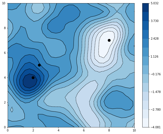
It easily fits the three datapoints, with a max and a min approximately centered around two of them that were purposely put in the prior’s tail.

Next steps

Of course GPs are a rich topic, and we are barely scratching the surface. On the mathematical front, some natural next steps would be in a few directions: 1) looking inward, explore more carefully the kernel, model selection, the Gaussian itself; 2) looking at connections between the GP and other models/structures, like the SVM, or Brownian motion; 3) looking at the GP’s use as a building block in other applications, for example in neural networks or stochastic processes (like the log-Gaussian Cox process).

On the coding front, it would be good to familiarize with some of the popular libraries for GPs, like sklearn’s or GPflow which uses Tensorflow, or several others listed here. It’s also natural to want to test drive this on some datasets, which we didn’t do here because this post is already way too long haha.

Thanks for reading!