Neural Networks for a beginner (Part I: theory)

Written on September 30th, 2017 by Steven Morse

Why neural networks?

The idea of an “artificial neural network” — that is, a networked series of transformations taking inputs and outputting a prediction — traces back to at least the 1950s as a way to explicitly model the function of the brain with a mathematical model. Interest in NNs has recently increased, with large NNs (so-called “deep learning”) at the core of algorithms in breaking news articles like beating humans at Go and self-driving cars. Below is a video of a NN learning to play an Atari game.

NNs are now so ubiquitous that even that actress from Twilight has a paper using them (credit Andrew Beam’s great post for this find).

This post will attempt to demystify the inner workings of this trend in machine learning by giving a rudimentary theoretical background on how NNs work. My aim is to make the material accessible to an elective-level undergraduate audience focusing in applied mathematics or computer science. Most of the exposition is based heavily on that in MIT’s course 6.867.

The setup

A neural network (NN) consists of many small, simple computational units called neurons or nodes that perform simple tasks. Each neuron takes a scalar input, passes it through some transformation (like a sigmoid, or many others, which we will cover later), and spits out a scalar output. The NN is in this sense a “black box”: we feed an input, it returns an output.

Our data consists of a set of pairs \(\{(x^{(i)}, y^{(i)})\}\) where \(x^{(i)}\) is the vector (ordered list) of scalar values for the \(i\)-th entry, and \(y^{(i)}\) is the corresponding target value. We typically consider \(x^{(i)}\in\mathbb{R}^d\), where \(d\) is the dimension of the independent variable, and denote the \(j\)-th feature of the \(i\)-th data point as \(x_j^{(i)}\).

Our target values \(y^{(i)}\) will either be scalar, i.e. \(y^{(i)}\in\mathbb{R}\), or they will take values from some finite set, i.e. \(y^{(i)}\in S\). The scalar case is called regression (think linear regression), while the finite-set case is called classification (since the set usually corresponds to different classes or types of points). We’ll focus on regression in this post, and classification in the sequel.

Our task is to develop a model such that given a previously unseen \(x^{new}\), we can accurately predict \(y^{new}\). We will assume we are given some block of data on which to train our model (the “training data”), and will be testing our model an unseen block of data (the “testing data”). And because this is a post about neural networks, we decide that the best model to use for this is … a neural network.

Feed-forward

First we feed the input forward through the NN, doing all the transformations at each node in each layer, until we reach the final layer which gives us our output. Of course, each of those transformations requires parameters, which we can set more or less randomly the first time through (more on this later). We will briefly describe this intuitive “feed-forward” process, before discussing the less-intuitive process of measuring how wrong our output was and feeding the correction back through the network to improve our NN.

(In this post we will only consider input that is a vector. We can generalize our input to matrices (for example, an image as input) later.)

A neural network consists of:

1. Input layer. This “receives” our input vector. Each node in the input layer corresponds to a single entry of the input vector.

2. Hidden layer(s). Each node in a hidden layer receives inputs from a previous layer, aggregates these inputs, and outputs some (simple) transformation of it. We often refer to the output of a neuron as its activation.

3. Output layer. This may be a single neuron or multiple. It receives the transformations of the last hidden layer, and outputs the prediction.

Example: single hidden layer

Consider a NN which takes inputs with \(d\) features, passes it through a single hidden layer of \(m\) neurons, and outputs a scalar value. Each layer is fully connected to the next.

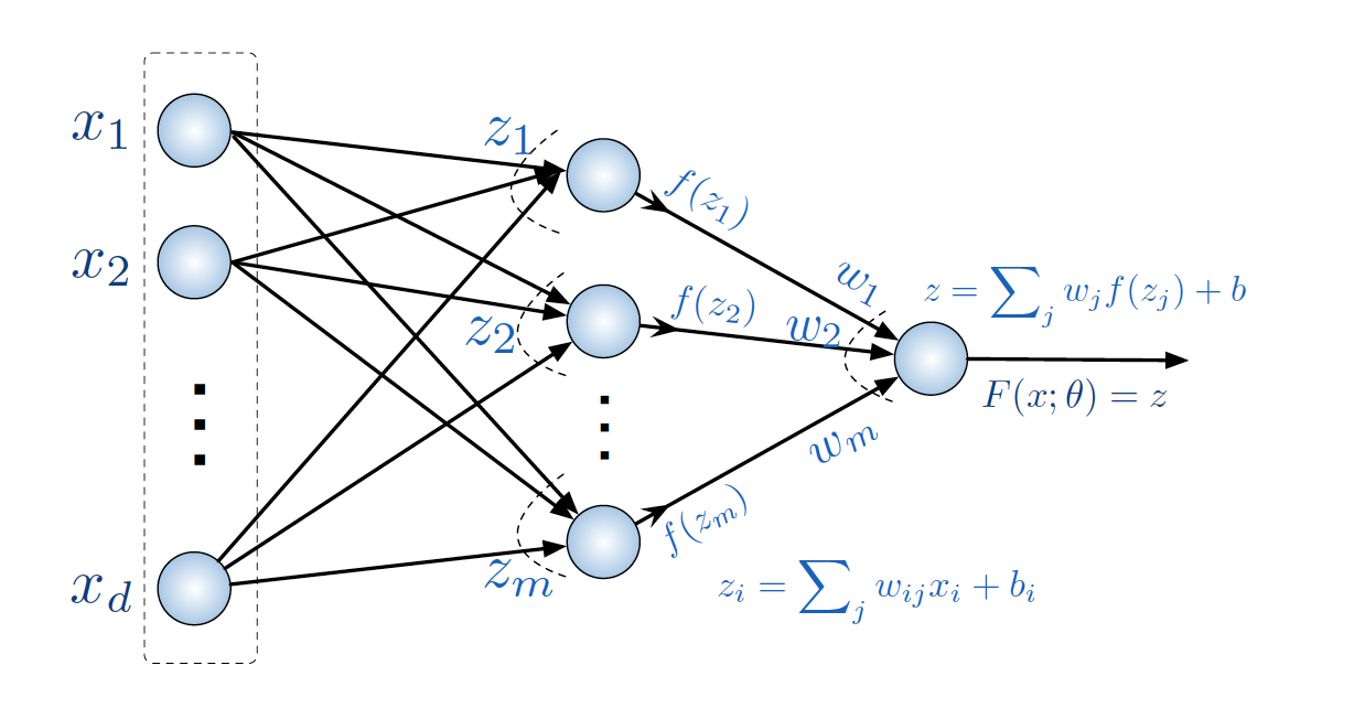
The input vector is \(x=(x_i)\). Then, each hidden layer neuron computes its output in two steps. First, each neuron does a linear transformation of the entire input layer, for example the \(i\)-th neuron computes:

\[\text{Aggregate:} \quad z_i = \sum_{j=1}^d w_{ij} x_i + b_i\]

according to weights \(w_{ij}\) such that \(i=1,...,m\) where \(m\) is the size of the hidden layer, and \(j=1,...,d\). The \(b_i\) is some intercept parameter (just like a linear regression). Then, the hidden layer neuron uses this scalar output \(z_i\) to perform its activation step:

\[\text{Activate:} \quad a_i = f(z_i)\]

where \(f(z_i)\) is the activation function of the neuron. Now note that if we make \(f(z_i)=z_i\), then each neuron is just a linear transformation of its inputs, and we’ll just get a giant linear regression! Instead, we typically use non-linear activation functions. Examples: the function \(f(z_i) = \text{max}(0, z_i)\) is called the rectifier and we would call this neuron a rectified linear unit or ReLU. Another popular choice is the sigmoid function \(f(z_i) = 1/(1+e^{-z_i})\). Intuitively, the ReLU “zeros out” any negative input (and does nothing to positive input), while the sigmoid transforms any input to the range \([0,1]\).

Finally, the single output neuron receives all these \(a_i\)’s and computes

\[z = \sum_{j=1}^m w_j a_i + b, \quad\quad F(x) = z\]

or in other words, does another linear transformation of all the ReLU activations according to weights \(w_j\) and intercept \(b\), then outputs this scalar value.

Training the NN

Now we have a black box built — how do we train it to give good outputs?

You are of course familiar with single variable linear regression, where we choose parameters for a line (slope and intercept) that minimize the sum of squared error between that line and the actual data.

We can take the same approach here. Let’s choose a loss function \(\ell(y, F(x))\) that computes the error between a target value \(y\) and our predicted value \(F(x)\) (i.e. the output of the last layer). For example, we might pick \(\ell(y,z)=\frac{1}{2}(y-z)^2\) (our familiar friend the squared error). Now, formally, we want to find a parameter estimate \(\hat{\theta}\) that minimizes the loss over all data,

\[\hat{\theta} \ = \ \text{arg}\min_{\theta} \quad \sum_{i=1}^n \ell(y^{(i)}, \ F(x^{(i)}))\]

where \(\theta\) refers to all the parameters of our black box, which is alllll the weights and intercepts assigned to each neuron. That’s a ton of parameters. What’s worse, whereas with linear regression we could solve this optimization problem analytically, we know that \(F(x)\) term is hiding a recursive list of a bunch of hidden layer activation functions which we’re not so sure will give rise to a closed formula. Also, whereas least squares is a convex optimization problem (meaning there is only one minimum and it is the global minimum), our neural network is non-convex (meaning there might be a lots of local minima before we find the global minimum).

Idea 1: Stochastic Gradient Descent (SGD)

The first trick we can hurl at this problem is to minimize our total loss using a numerical optimization technique called stochastic gradient descent.

You are probably familiar with basic gradient descent. This is the idea that, given some function \(f(x)\) (where \(x\) may be a vector), we can navigate to a minimum by pointing in the direction of steepest descent (i.e. the direction of the negative gradient), taking a carefully sized step, then repeating. Eventually we will reach a minimum, and if our function is convex, it will be the global minimum.

Stochastic gradient descent (SGD) is a version of this method that we can use when the function we are minimizing is actually a sum of functions. Like, for example, our sum of the loss function on each data point. In SGD, we just take a step in the direction of steepest descent at a particular data point. So each step is:

\[\theta = \theta - \eta \nabla_{\theta} \ell(y^{(i)}, F(x^{(i)}))\]

A cautionary note here: don’t forget that our domain is the parameter space, \(\theta=(\theta_i)\). We are used to seeing \(x\) as the domain and \(y\) as the range, but in this case (and as is typical in machine learning), the \(x\)’s and \(y\)’s are static datapoints, and it is the \(\theta\)’s that we are moving around in (the domain), measuring our progress in terms of \(\sum_i \ell(y^{(i)}, F(x^{(i)}))\) (the range).

A second cautionary note: don’t forget that \(\theta\) is a vector of all our parameters, and the gradient \(\nabla_{\theta} \ell\) is a vector of partial derivatives with respect to each of those different parameters.

What is magical about SGD is that we can take a step like this at some random data point, update our parameter estimate \(\theta\), then pick any other random data point and do it again, iterating. And magically, we will eventually converge to a minimum. (Well, as long as some conditions are met such as tuning our learning rates \(\eta\) correctly..)

Sidenote: There is growing evidence that one reason neural networks work so well, or more specifically, the reason they do not overfit despite their enormous number of parameters, is due to the tendency of SGD to find “flat” optimums, as opposed to “pointy” ones.

Example

Let’s use our example from before and take a swag (Scientific Wild Ass Guess) at that gradient \(\nabla_{\theta} \ell(y, F(x))\) for some particular datapoint \((x,y)\) (note this is a single datapoint, just simplifying notation). We’ll look at just the partial derivative with respect to a single weight \(w_{ij}\), which recall is the value of the \(j\)-th element of the \(i\)-th neuron’s linear transformation.

Let’s list the series of transformations/functions/activations from start to finish of our neural network:

\[\begin{align*} z_j &= \sum_{i=1}^d w_{ij} x_i + b_j \quad \text{(input to j-th neuron)}\\ f(z_j) &= \text{max}(0, z_j) \quad \text{(output of j-th neuron)}\\ z &= \sum_{j=1}^m w_j z_j + b \quad \text{(input to final output neuron)} \\ f(z) &= F(x) = z \quad \text{(final output)} \end{align*}\]

So to take the partial derivative of \(\ell(y, z)\) w.r.t. some weight \(w_{ij}\) we can apply the chain rule and get:

\[\frac{\partial \ell(y, z)}{\partial w_{ij}} = \left[ \frac{\partial z_j}{\partial w_{ij}} \right] \left[ \frac{\partial f(z_j)}{\partial z_j} \right] \left[ \frac{\partial z}{\partial f(z_j)} \right] \left[ \frac{\partial \ell}{\partial z} \right]\]

Now this is encouraging. These are all very tractable partial derivatives: for example, the partial of \(z_j\) w.r.t. \(w_{ij}\) is just \(x_i\). Depending on our choice of activation function \(f(z_j)\) or loss function \(\ell(y, z)\) we might have to resort to something called subgradients, but for now let’s assume we can write down all these partial derivatives and feel good about ourselves.

Idea 2: Back-propagation

We still have a problem though. With potentially dozens of layers and hundreds/thousands of neurons, we have a combinatorial explosion of gradients to compute.

There is hope. The second trick, our finishing move, is to trade time for space (memory). If we can save in memory the inputs \(z\) and activations \(a\) at each step, then computing the gradient of the loss w.r.t. some parameter is a one-step, self-contained formula.

To make our derivation a little easier to follow we introduce some vector notation. First, denote the parameters \(w_{ij}\) for a particular hidden layer \(l\) as the matrix \(W^l=(w_{ij}^l)\). This is a natural choice: each neuron in a hidden layer corresponds to a column, and each element of the input vector corresponds to a row. Then also:

\[\begin{align*} a^{l-1} &= (a_1^{l-1}, ..., a_m^{l-1}) \quad \text{(activations of layer } l-1 \text{ with } m^{l-1} \text{ neurons)}\\ z^l &= (W^l)^T a^{l-1} + b^l \quad \text{(aggregated inputs of layer l)} \\ a^l &= f(z^l) \end{align*}\]

So we have collected all the weights of layer \(l\) into a matrix \(W^l\) such that the \(j\)-th column are the \(m\) weights for the \(j\)-th neuron.

Now, we need to compute \(\partial \ell / \partial \theta\), i.e. the partial derivative with respect to each parameter of the model. Let’s consider just \(\partial \ell / \partial W^l\) for some layer \(l\).

\[\frac{\partial \ell}{\partial W^l} = \frac{\partial z^l}{\partial W^l} \frac{\partial \ell}{\partial z^l} = \frac{\partial z^l}{\partial W^l} (\delta^l)^T\]

Here we just defined \(\delta^l = \frac{\partial \ell}{\partial z^l}\), the change in loss w.r.t. the layer \(l\). Note also that \(\frac{\partial z^l}{\partial W^l} = a^{l-1}\).

Now we sense we may be able to establish some recursion for \(\delta^l\). Let’s write

\[\frac{\partial \ell}{\partial z^l} = \frac{\partial z^{l+1}}{\partial z^l} \frac{\partial \ell}{\partial z^{l+1}} = \frac{\partial z^{l+1}}{\partial z^l} \delta^{l+1}\]

and since we know

\[z^{l+1} = (W^{l+1})^T a^l + b^{l+1} = (W^{l+1})^T f(z^l) + b^{l+1}\]

we can differentiate w.r.t. \(\partial z^l\) and obtain

\[\frac{\partial z^{l+1}}{\partial z^l} = \text{diag}(f'(z^l))(W^{l+1})\]

where \(\text{diag}(f'(z^l))\) is the diagonal matrix formed from the vector \(f'(z^l)\). Substituting this into what we had before, we write

\[\delta^l = \frac{\partial \ell}{\partial z^l} = \text{diag}(f'(z^l)) W^{l+1} \delta^{l+1}\]

and we have a recursion. So, from a layer \(l\), we could follow this all the way forward to the final layer \(L\) as

\[\delta^l = \text{diag}(f'(z^l)) W^{l+1} \delta^{l+1} \text{diag}(f'(z^{l+1})) W^{l+2} ... W^L \delta^L\]

and the last layer is \(\delta^L = \partial \ell / \partial z^L = \text{diag}(f'(z^L))\partial \ell / \partial a^L\).

Summary

Altogether, the procedure for training a NN is to

1. Input a training pair \((x, y)\) and set “activations” in the input layer as \(a^1 = x\)

2. Feedforward. For each \(l=2,3,...L\), compute the aggregation and activation at each neuron in each hidden layer.

3. Output layer error. Compute the gradient of the loss at the last layer, \(\delta^L =\text{diag}(f'(z^L))\partial \ell / \partial a^L\)

4. Backpropagation. For each \(l=L-1, ..., 2\) compute \(\delta^l = \text{diag}(f'(z^l)) W^{l+1} \delta^{l+1}\).

5. Gradient. With this information in hand, we can compute the gradients \(\partial \ell / \partial W^l = a^{l-1}(\delta^l)^T\) and \(\partial \ell / \partial b^l = \delta^l\).

6. Gradient step. Using the gradients, take a (stochastic) gradient step and update the parameters based on the training pair. Return to step 1.

Practical considerations

A few quick implementation considerations:

1. Initializing the weights. Since the loss function is highly nonconvex, it is essential to take care in initializing our startpoint, i.e., our initial parameter values. For example, when using ReLUs, if we initialize all our weights to zero, then all our activation function inputs will always be zero and therefore our outputs will always be zero and will never change despite any number of training data. One better choice is to initialize the weights by sampling from a Gaussian distribution with mean zero and variance based on the number of neurons in a particular layer (for example, setting variance \(\sigma^2 = 1/m\)). It can be shown that this causes the variance of the output to varies in proportion to the variance of the input.

2. Regularization. The enormous number of parameters inherent to a NN encourages “overfitting” to the training data. As mentioned, SGD may help prevent this, but another technique is to introduce a regularizer in our loss function, for example by penalizing large weights by adding a norm on the weights to the loss function.

3. Dropout. Another popular type of regularization is called “dropout,” where we randomly turn-off neurons during training. In this scheme, neurons rely on signals from their neighbors on the importance of particular connections. This methodology requires adjustments to both the feedforward and backprop implementations.

Further reading

There are many other fine tutorials around the web for dipping one’s toe in the water of neural networks, most of them more detailed than the one presented here. My aim was not to be thorough, but friendly, and to cover all the relevant ideas in a short, digestible post. If you know of other good resources for my intended audience (undergraduates), I’d be happy to add them here, please contact me via email or Twitter. Thanks for reading!

Written on September 30th, 2017 by Steven Morse