Neural Networks for a beginner (Part II: code)

Let’s implement the ideas from this post in Python to create a working, customizable neural network (NN). Then we’ll test it on two classic didactic datasets, an XOR dataset and the the MNIST handwritten digits. This particular implementation will therefore focus on classification, although the code could be easily modified to perform regression instead. We’ll be a using exclusively NumPy, and the base time package to track progress:

import numpy as np
import time as T

Class shell

Let’s take an object-oriented approach and use a Python class to encode an instance of a particular NN. (This follows the methodology of sklearn.) The shell of the class we’ll setup as:

class NN:
    def __init__(self, f, gf, F, hdims=[4]):
        self.f = np.vectorize(f)
        self.gf = np.vectorize(gf)
        self.F = F
        self.dims = hdims
        self.nlayer = len(hdims)+2
        self.model = {}

    def train(self, X, Y, stop_criterion='max_epochs', Xv=None, Yv=None, tol=0.02,
              max_epochs=100, tau0=1000, kappa=0.7, verbose=False):
        # TO DO

    def predict(self, x):
        # TO DO

The inputs to our neural network class NN are the activation function f, its gradient gf, and the output layer activation F. We also need to specify the size of each hidden layer as a list hdims, with the default being one hidden layer of size 4. (Note this requires us to use the same activation function throughout each hidden layer.)

These are stored in the class instance, along with a dict named model which will store the parameter estimates themselves.

The rest of the class consists simply of a train and a predict method. The train method takes in training data X, labels Y, and various SGD details which we will cover in more detail later. The predict method simply takes a set of inputs x and should return the predicted labels.

Separately, we will define some activation functions and their gradients:

def relu(z): 
    return np.max([0, z])

def g_relu(z): 
    return 1 if z > 0 else 0

def softmax(z): 
    s = np.sum(np.exp(z))*1.0
    return np.exp(z) / s

Train

The train method implements a feedforward-backprop loop over the data, following the steps at the end of the previous post. Let’s take a look at the code, and then talk through some of the trickier parts.

def train(self, X, Y, stop_criterion='max_epochs', Xv=None, Yv=None, tol=0.02,
              max_epochs=100, tau0=1000, kappa=0.7, verbose=False):
        N, d = X.shape
        
        # dims = [d, z2, z3, z4, ..., out]
        self.dims.insert(0, X.shape[1])
        self.dims.append(Y.shape[1])
        dims = self.dims
        nlayer = self.nlayer
        
        # W, b = [W2, W3, ...]
        W = [np.random.normal(0, 1./dim, dim*dimp1).reshape(dim,dimp1) \
             for dim,dimp1 in zip(dims[:-1], dims[1:])]
        b = [np.random.normal(0, 1, dim) for dim in dims[1:]]

        k = 0
        START = T.time()
        prevacc = 0.0
        for ep in range(max_epochs):
            if verbose and ep%100==0: print('Epoch %d, Elapsed: %1.3f' % (ep, T.time()-START))
            for n in np.random.permutation(range(N)): 
                # feed forward
                z = [[] for _ in range(nlayer-1)]   # z = [    z2, z3, ..., zL] 
                a = [[] for _ in range(nlayer)]     # a = [a1, a2, a3, ..., aL]
                a[0] = X[n]
                for i in range(nlayer-1):
                    z[i] = (W[i].T).dot(a[i]) + b[i]
                    a[i+1] = self.f(z[i]) if i < nlayer-2 else self.F(z[i]) 
                
                # back prop
                d = [[] for _ in range(nlayer-1)]   # d = [d2, d3,..., dL]  
                d[-1] = a[-1] - Y[n]
                for i in reversed(range(nlayer-2)):
                    d[i] = np.diag(self.gf(z[i])).dot(W[i+1]).dot(d[i+1])
                
                # SGD
                eta = np.power((tau0 + k), -kappa) # Robbins-Monro. alt: kappa/(k+1)
                for i in range(0, nlayer-1):
                    W[i] += -eta * ((a[i].reshape(dims[i],1)).dot(d[i].reshape(1,dims[i+1])))
                    b[i] += -eta * d[i]
                
                k += 1
            
            # stopping criteria
            if stop_criterion=='validation' and ep % 10 == 0:
                self.model = {'W': W, 'b': b}
                curacc = self.score(Xv, Yv)
                if verbose: print(' - (prevacc=%1.2f) (curacc=%1.2f)' % (prevacc, curacc))
                if curacc <= prevacc - tol:
                    if verbose: print('Reached stopping criterion.')
                    break
                else:
                    prevacc = curacc
                
        if verbose: print('Total Elapsed: %1.3f' % (T.time()-START))
            
        self.model = {'W': W, 'b': b}

Inputs to train are our data X with labels Y, then stopping criterion for SGD which may either be based on a fixed number of iterations through the data (max_epochs) or a plateau in increasing accuracy on a validation dataset, specified as Xv, Yv, and tol. The tau0 and kappa parameters govern our SGD stepsize using the Robbins-Monro criteria of

where \(k\) is the current iteration index. We will typically select \(\tau_0\) as some large number, and \(\kappa\in[0.5,1]\). We then initialize our weights W and intercepts b by sampling from a mean-zero Gaussian distribution with variance \(\sigma^2 = 1/m\) as described in the previous post.

The meat of the train method is in two nested for-loops, where we loop over each epoch, and then randomly over each datapoint, one at a time. At each datapoint, we first feedforward the input by performing aggregation and activation at each hidden layer. We then compute the gradients for each weight and intercept using the backprop procedure outlined previously. Finally, we update each parameter with the adaptive learning rate \(\eta\).

If we set our stopping criteria to “validation,” we will check our current accuracy on the validation set against our previous. There are many possible variations on stopping criteria for SGD, we are only showing two here. This stopping criterion uses the score method, since we are assuming we are doing classification. score in turn uses the predict method, which we cover next.

Predict

The predict method, and the accompanying score method, are as follows.

def predict(self, x):
    z = [[] for _ in range(self.nlayer-1)]
    a = [[] for _ in range(self.nlayer)]
    a[0] = x
    for i in range(self.nlayer-1):
        z[i] = (self.model['W'][i].T).dot(a[i]) + self.model['b'][i]
        a[i+1] = self.f(z[i]) if i < self.nlayer-2 else self.F(z[i]) 
    return a[-1]
    
def score(self, Xt, Yt):
    return np.sum(1 if np.argmax(self.predict(xi))==np.argmax(yi) else 0 \
                  for xi,yi in zip(Xt,Yt)) / float(len(Xt))

The predict method is as simple as a feedforward pass through the network using the current parameters W and b. In fact, you could probably make a “feedforward” function and call it for both train and predict, but that sounds like a tweak for another day! The score method assumes we have used a 1-hot encoding scheme for our labels.

Sidenote: 1-hot encoding simply means that if \(y\in \{0,1,2\}\), and \(y^{(i)}=2\), then we set \(y^{(i)}=(0,0,1)\).

Case study 1: XOR Dataset

A classic test of a classifier is the XOR dataset. This is any dataset where the data forms a kind of \(2\times 2\) checkerboard pattern — the simplest example would be the dataset:

x1 = (0, 0), y1 = (0)
x2 = (0, 1), y2 = (1)
x3 = (1, 0), y3 = (1)
x4 = (1, 1), y4 = (0)

This gets its name due to the labels being the logical exclusive-or (XOR) of the inputs. We’ll construct a larger example by generating points randomly distributed around the centers (2,2), (2,-2), (-2,-2), and (-2,2), with the appropriate XOR classes.

We now have a binary classification problem that is not linearly separable, thus making linear classifiers like logistic regression or SVMs (without a change of basis or use of kernel methods) impractical, and therefore providing a nice proving ground for our NN.

We generate some XOR data and split it into training, validation and test, with a 50-25-25 split. We load this data then as X, Y, Xv, Yv, and Xt, Yt. We train our NN method using the validation set as stopping criterion, as follows:

net = NN(relu, g_relu, softmax, hdims=[10])
net.train(X, Y, stop_criterion='validation', Xv=Xv, Yv=Yv, tol=0.01, max_epochs=400, verbose=True)

Epoch 0, Elapsed: 0.000
 - (prevacc=0.00) (curacc=0.93)
 - (prevacc=0.93) (curacc=0.94)
 - (prevacc=0.94) (curacc=0.94)
 - (prevacc=0.94) (curacc=0.95)
 - (prevacc=0.95) (curacc=0.95)
Total Elapsed: 7.123

We can plot the resulting classification boundary on the test data, along with our test accuracy, with the following pyplot code:

def plotDecisionBoundary(X, Y, nn, values=[0.05, 0.5, 0.95], title=''):
    x_min, x_max = X[:,0].min() - 1, X[:,0].max() + 1
    y_min, y_max = X[:,1].min() - 1, X[:,1].max() + 1
    h = max((x_max-x_min)/200., (y_max-y_min)/200.)
    xx, yy = np.meshgrid(np.arange(x_min, x_max, h),
                         np.arange(y_min, y_max, h))
    zz = np.array([nn.predict(x)[0] for x in np.c_[xx.ravel(), yy.ravel()]])
    zz = zz.reshape(xx.shape)

    # plot margins as contour(s)
    CS = plt.contour(xx, yy, zz, values, 
                     colors='black', linestyles=['dotted', 'solid', 'dotted'], 
                     linewidths=[1,2,1])
    plt.clabel(CS, fontsize=9, inline=1, fmt='%1.2f')

    # plot data
    colors = ['b' if np.argmax(yi)==1 else 'y' for yi in Y]
    plt.scatter(X[:,0], X[:,1], c=colors, alpha=0.5)

    plt.xlabel('$x_1$', fontsize=16)
    plt.ylabel('$x_2$', fontsize=16)
    plt.title(title, fontsize=18)

This will give us not only the classification boundary — i.e., where the neural network is \(>50\%\) sure data is in one class or another — but gives us an indication of the 95% probability region too. The tighter this is to the 50% divider, the more “confident” our model is. The resulting plot is shown below.

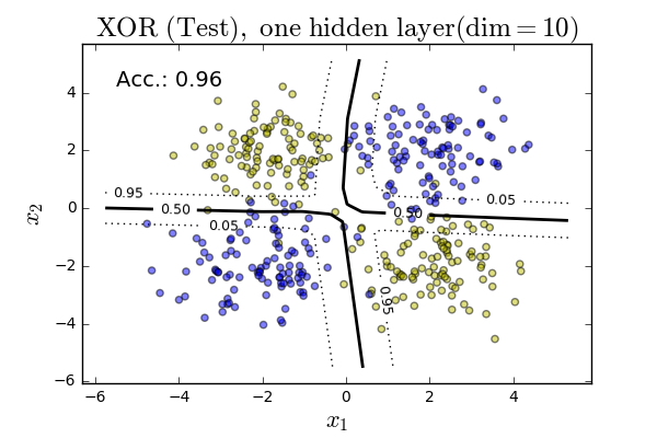
Note our “architecture” for this data was very simple: our input layer, corresponding to the data, was two neurons. We then had a single hidden layer of only 10 neurons, using ReLU activations. Finally, we had two neurons in the output layer to account for our binary classification task. With this relatively simple architecture, we were able to achieve 96% accuracy on the test set for this canned, but illustrative example.

Case study 2: MNIST Handwritten Digit Recognition

Now let’s try a more interesting example: the MNIST dataset. This database of images of handwritten digits has been a mainstay of testing machine learning and image processing algorithms for many years (the original NIST data dates back to the mid-1990s). Each datapoint consists of a 28x28 grayscale pixel capture of a human’s handwritten digit, and the associated actual digit being written. The data is hosted by Yann LeCun, and due to its ubiquity as an ML benchmark, tutorials abound for using it.

As opposed to going down the rabbit hole of convolutional neural networks or other more sophisticated ways to handle image processing and “computer vision,” let’s collapse each 28x28 image into a single vector of length 784. We will encode the 10 class labels with a 1-hot encoding.

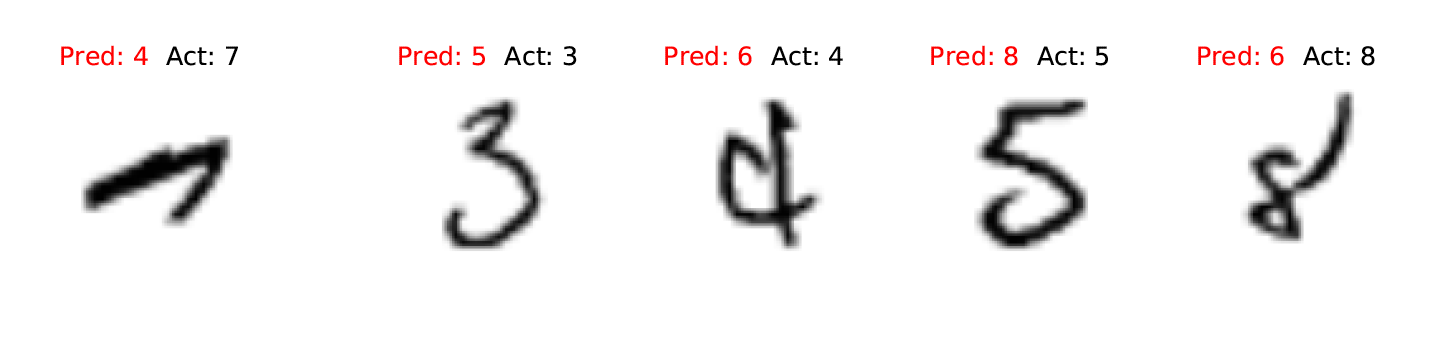
We load the data, normalize it (try doing the classification without normalizing — what happens? why?), and train on 1,000 examples of each digit. As our architecture we again choose a single hidden layer, this time of 20 neurons. We achieve 99% accuracy on the training set, and, perhaps surprisingly, 97% accuracy on the test set! Let’s take a look at some of our misclassified digits.

Further reading

This is a tiny skeleton of a neural network framework. The aim was not to develop a rigorous product, but to develop a working one that gives some insight into the inner workings of a neural network without getting bogged down in production level code optimizations and error checking.

Besides, due to the interest in the subject, there are many, many more sophisticated frameworks already out there, in your programming language of choice. I’ll mention the two that I think are the most well-known and best documented, but of course there are many others. First, the TensorFlow project, which offers an extremely powerful API and is both beginner and expert friendly. Second, a more Python-specific package that also uses GPU acceleration is PyTorch. Both have some excellent tutorials and are worth checking out.

I hope you’ve enjoyed this two-part tutorial, and I welcome any feedback.