Elo as a statistical learning model

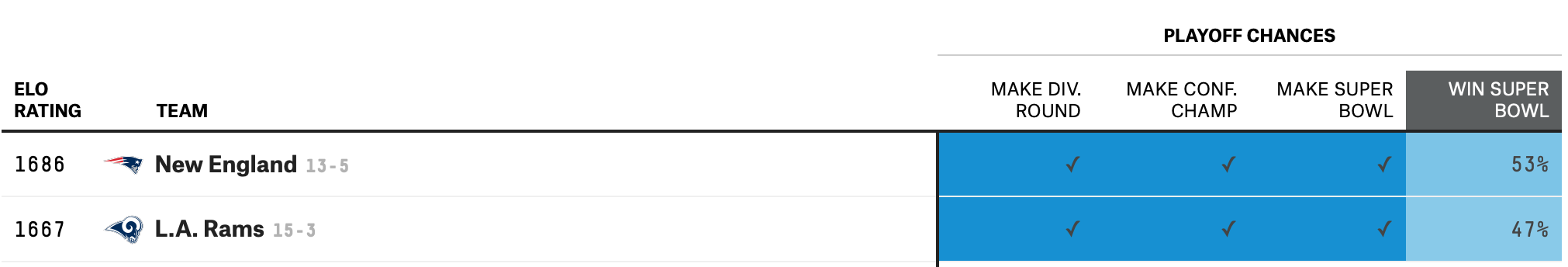
Written on May 20th, 2019 by Steven Morse

Elo ratings are a ubiquitous system for ranking individuals/teams who compete in pairs. They began as a chess rating system, designed by Arpad Elo, but have since spread to sports and elsewhere (here’s an application in education). As a result, there is a lot of info out there on how to compute Elo ratings, presumably because they’re easy to understand and surprisingly good at forecasting. Heck, pretty much all of Nate Silver’s 538 sports coverage revolves around it. Here’s their forecast going into the last Superbowl … I guess they called it?

But there are very, very few resources on how the ratings work. I don’t mean what the formula is, I mean why the formula is what it is. What is the deeper statistical truth going on here?

I’m going to take a schwack at this. I’ll explore the Elo ratings as weights of a logistic regression found through stochastic gradient descent. A few other resources mention or hint at this interpretation, but their explanations feel cursory at best to me. (This also helps me connect Elo to its more typical framing as an AR(1) autoregressive process, where things like 538’s autocorrelation adjustment come in, since SGD is itself interpretable this way too.)

My hope is that placing Elo in a statistical learning framework will allow us to extend it, or improve it.

CAVEAT: An ulterior motive of this post is to lure the casual sports analytics enthusiast into a deeper understanding of stats, so if you have a PhD in statistics and a lot of this seems pedantic … my bad. (Also, if you find errors, let me know!)

Elo: a quick primer

Let’s say Team \(i\) and Team \(j\) have Elo ratings \(\text{elo}_i\) and \(\text{elo}_j\). They play a game against each other. This results in the update

\[\begin{equation} \text{elo}_{i}^{(\text{new})} = \text{elo}_{i}^{(\text{old})} + k (t_{ij} - \text{Pr}(i \text{ beats } j)) \label{eq:elo} \end{equation}\]

and the corresponding update for \(j\). Here \(k\) is the “k”-factor, \(t_{ij} = 1\) if \(i\) beats \(j\) (0 otherwise) is the game outcome, and \(\text{Pr}(i \text{ beats } j)\) is the probability that \(i\) wins the game. The k-factor captures how much impact a single game has on the ranking, so for example, 538 uses 20 for NFL games and 4 for MLB games. The probability of winning is defined as a weird base-10 sigmoid function of the difference in ratings:

\[\text{Pr}(i \text{ beats } j) = \frac{1}{1+10^{-(\text{elo}_i - \text{elo}_j)/400}}\]

That 400 is typically described as a “scale factor” (but why 400?). The base 10 comes because, for whatever reason, Arpad Elo decided to use \(\log_{10}\) odds instead of the typically \(\log_e\) odds.

For games with point spreads, we can also use Elo ratings to predict the spread: each game point corresponds to 25 Elo points (but why?).

Logistic regression

This should all remind us of logistic regression. As a quick and dirty review, let’s say we have some data \(\mathcal{D}=\{(\mathbf{x}_i, y_i)\}\) where \(\mathbf{x}_i\in\mathbb{R}^d\) and \(y_i\in\{0,1\}\). We are interested in predicting an outcome \(y\) given input \(\mathbf{x}\).

First recall “odds” is defined as the probability of something happening divided by the probability it doesn’t (so 3:1 odds implies the thing has a 75% chance, since 0.75/0.25 = 3). Now define the “log-odds”

\[a = \log \frac{\text{Pr}(\mathbf{x}| y=1)\text{Pr}(y=1)}{\text{Pr}(\mathbf{x}| y=0)\text{Pr}(y=0)}\]

where we typically assume \(\log = \log_e\). Then note, by Bayes’ theorem,

\[\begin{align*} \text{Pr}(y=1|\mathbf{x}) &= \frac{\text{Pr}(\mathbf{x}| y=1)\text{Pr}(y=1)}{\sum_k \text{Pr}(\mathbf{x}| y=k)\text{Pr}(y=k)} \\ &= \frac{1}{1+\frac{\text{Pr}(\mathbf{x}| y=0)\text{Pr}(y=0)}{\text{Pr}(\mathbf{x}| y=1)\text{Pr}(y=1)}} \\ &= \frac{1}{1+e^{-a}} \end{align*}\]

This is the workhorse “sigmoid” function, usually written \(\sigma(a)\).

(And doesn’t it remind you of the Elo rating probability??)

If we now assume the log-odds can be written as a linear combination of the inputs \(\mathbf{x}\) (or more probabilistically, if we assume the conditional densities are Gaussian with a shared covariance matrix and equally likely classes), then

\[\text{Pr}(y=1 | \mathbf{x}; \mathbf{w}) = \sigma(\mathbf{w}^T \mathbf{x})\]

for some “weight” vector \(\mathbf{w}\). Then the data likelihood can be written

\[\text{Pr}(\mathcal{D}|\mathbf{w}) = \prod_{i=1}^N \sigma^{y_i} (1-\sigma)^{1-y_i}\]

which we’d like to maximize, or equivalently the negative log-likelihood

\[E(\mathbf{w}) := -\log \text{Pr}(\mathcal{D}|\mathbf{w}) = -\sum_{i=1}^N y_i \ln \sigma + (1-y_i) \ln (1-\sigma)\]

called the “cross-entropy,” which we’d like to minimize. Since \(\partial_{\mathbf{w}} \sigma = \sigma (1-\sigma)\) (so nice!), the gradient turns out to be

\[\begin{equation} \nabla_{\mathbf{w}} E = \sum_{i=1}^N (\sigma(\mathbf{w}^T \mathbf{x}_i) - t_i) \mathbf{x}_i \label{eq:entropy_grad} \end{equation}\]

which you should verify on a piece of scrap paper sometime when you’re feeling frisky.

(Notice each term in the sum here kinda looks like the \((1-\text{Pr}(i))\) term from the Elo update in Eq. \eqref{eq:elo} — more on this in a bit.)

There isn’t a closed-form solution to Eq. \eqref{eq:entropy_grad} like there is for, say, linear regression, but we can readily apply a numerical technique like gradient descent.

Image credit: Golden

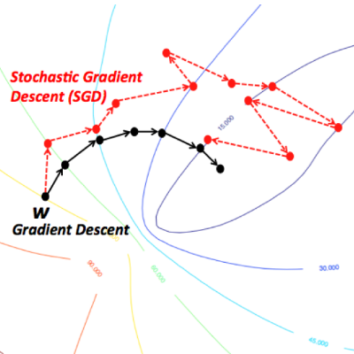
Stochastic Gradient Descent

Gradient descent is the beautifully simple technique of looking for a minimum by taking small steps in the direction of the negative gradient, that is,

\[\begin{equation} \mathbf{w}_{k+1} = \mathbf{w}_k - \alpha \ \nabla E(\mathbf{w}_k) \end{equation}\]

where \(\alpha\) controls how fast we update our estimate of \(\mathbf{w}\) (and could be adaptive, i.e. depend on \(k\)).

(Storytime: “first order” methods like gradient descent — so-called because they only use the first order derivatives, as opposed to second-order methods like Newton-Raphson — were once dismissed as too simplistic and slow, but found redemption in the age of big data (we need it to be simple!) and fast computers (not slow anymore!).)

Now notice, when the dataset is very large, the sum happening in \(\nabla E\) is very large, and so we are evaluating a very large function at every step of the algorithm.

It turns out, you can just evaluate the gradient at one of the terms in the sum, and move in that direction, and you will still provably reach a minimum, so long as you keep picking random terms and you do it enough times! This is absolutely magical to me.

This is called stochastic gradient descent, and so for logistic regression would look like

\[\begin{equation} \mathbf{w}_{k+1} = \mathbf{w}_k - \alpha \ \big(\sigma(\mathbf{w}_k^T \mathbf{x}_i) - t_i \big) \mathbf{x}_i \label{eq:SGD} \end{equation}\]

This is looking eerily familiar. We’re almost there.

A connection

Let’s connect Elo to all this. For a concrete running example, consider the NFL. The weight vector \(\mathbf{w}\) is now the ratings of all 32 teams. Let’s denote a specific game between teams \(i\) and \(j\) as the datapoint \((\mathbf{x}_{(ij)}, y_{(ij)})\), where

\[\mathbf{x}_{(ij)} = [x_k] = \begin{cases} 1 & k=i \\ -1 & k=j \\ 0 & \text{otherwise} \end{cases}\]

and \(y_{(ij)} = 1\) if \(i\) wins, 0 if \(j\) wins. The class conditional probability of \(i\) winning is then

\[\text{Pr}(y_{(ij)}=1 | \mathbf{x}_{(ij)}; \mathbf{w}) = \sigma(\mathbf{w}^T \mathbf{x}_{(ij)})\]

since \(\mathbf{w}^T \mathbf{x}_{(ij)} = w_i - w_j\) or in Elo notation, \(\text{elo}_i - \text{elo}_j\). Then given some initial estimate of the weight vector \(\mathbf{w}_0\), we can hone our estimate of the weights by iteratively applying an SGD step on the data,

\[\mathbf{w}_{k+1} = \mathbf{w}_k - \alpha \ (\sigma (\mathbf{w}_k^T \mathbf{x}_{(ij)}) - 1) \mathbf{x}_{(ij)}\]

or being a little more explicit,

\[\begin{bmatrix} w_1 \\ ... \\ w_i \\ w_j \\ ... \\ w_N \end{bmatrix}_{k+1} = \begin{bmatrix} w_1 \\ ... \\ w_i \\ w_j \\ ... \\ w_N \end{bmatrix}_{k} + \alpha \left(1 - \frac{1}{1+e^{-(w_i - w_j)}}\right) \begin{bmatrix} 0 \\ ... \\ 1 \\ -1 \\ ... \\ 0 \end{bmatrix}\]

Take a second and confirm: the only two lines where anything’s going on out of this update correspond to the two Elo update equations for a game up in Eq. \eqref{eq:elo}. Lots of signs flipping back and forth, and don’t forget \(\sigma(-a)=1-\sigma(a)\), but they’re the same!

(Yes, instead of log-odds defined \(a=\log_e\), Elo uses \(a=400\log_{10}\), but this amounts to a rescaling.)

This sparse input vector thing I haven’t seen elsewhere, and it does seem weird. It seems strange that you could encode the entire dataset with \(y_i=1\), and it seems strange that the effective space of the input data is strictly less than the original dimension.

Anyway, from a high level, Elo ratings are actually weights of a logistic regression to predict pairwise game outcomes, which we learn through SGD-like updates over streaming data.

Next up

This was a quick look at a statistical learning interpretation of the Elo rating system. Some other topics I’d like to explore:

• 538’s ratings incorporate margin of victory and an autocorrelation remediation term in their learning rate \(\alpha\). Margin of victory seems to fit in as a use of “side-information” to create an adaptive learning rate. The autocorrelation factor is better understood as a correction term with Elo as an autoregression. I get the idea of why this term should be here, but not why 538 chose the form it uses.

• A typical extension to SGD is doing a sum over some of the terms in \(\nabla E\), called a “mini-batch.” Technically, doing all the Elo updates for a week of NFL football counts as a minibatch, but not in spirit, since it gives us the same parameter estimates as before. What happens if we batch entire months, or seasons?

• A common improvement to first order methods like GD/SGD is incorporation of momentum. (Here’s a beautiful Distill.pub article about it.) A simple example is the following modified gradient step:

\[\mathbf{w}_{k+1} = \mathbf{w}_k - \alpha \ \nabla E(\mathbf{w}_k) + \beta (\mathbf{w}_k - \mathbf{w}_{k-1})\]

Now, if we took a large “step” on our last update, we will take a large-ish step again, even if our gradient is small. This helps propel us through potentially long, flat portions of the error function surface. In the context of Elo ratings, this amounts to giving a team a little bump in ratings even if they had an unimpressive victory, so long as they had a blowout victory the week before.

• Whether we interpret Elo as an AR(1) process or an SGD update, there is an implicit assumption that each team has some “true” rating that we are trying to learn, which stays constant throughout each season. This is certainly too strong, but how much would it help to incorporate a changing underlying rating? Here’s a state-space, generative model by Mark Glickman that accounts for changing team abilities.

Written on May 20th, 2019 by Steven Morse