2 - Peeking under the hood with a linear model

Series: A (Slightly) Technical Intro to AI

AGI, Specialized AI, and Machine Learning: the big ideas
Peeking under the hood with a linear model
Expanding the framework: bigger data, bigger models
Getting crazy: (Deep) neural networks
A Safari Tour of Modern ML Models
Ethics, Limitations, and the Future of AI

In the previous post we introduced the 10,000 foot concept of most specialized AI: in short, they are flexible mathematical models that we can train to take inputs of a certain kind of data and produce correct outputs.

This is all fine but we still have no idea how the actual models, like, work. We’ve essentially explained how a car works by saying it’s a black box that takes in gas and air and outputs rotational motion. Now let’s talk about the internal combustion engine.

The following discussion is the most technical of the series, and you could skip it if the math seems intimidating. But it really isn’t that technical! And the math is why you’re reading this in the first place, right??! And in Part 3 and Part 4, we’ll show you can extend this idea to much more powerful models.

So read on.

A humble little model

In the last post, we thought about training an AI to correctly label images of dogs and cats. Now let’s say we are 15 years old, we run a neighborhood lawn mowing service, and we want to “train an AI” to predict the amount of money we will make this summer (call this $y$) given how much we spent on advertising flyers (call this $x$). Hopefully it’s enough to buy a used truck and expand our business next year.

The only thing we love more than mowing lawns is collecting data, and so we have historical data going back 6 years:

Lawnmowing Historical data

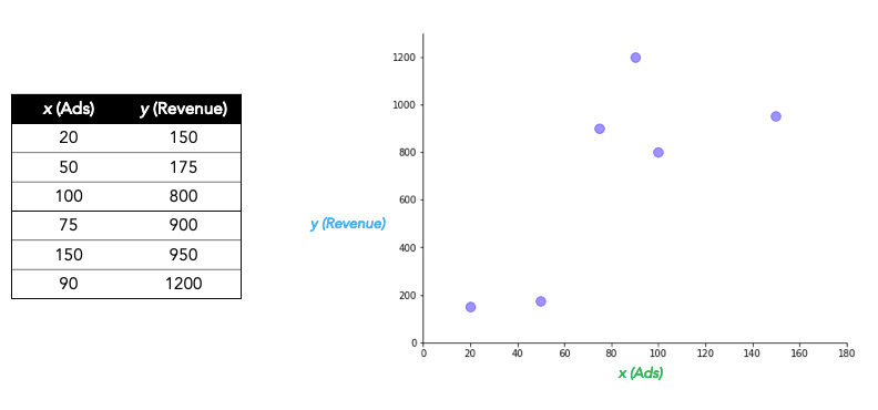
Step 0. Select a model.

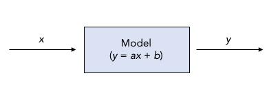
Upon inspection of the data, for our highly advanced ML prediction model, we decide to select … drumroll … a straight line! Specifically, our magic black box AI is

\[y = ax + b\]

where $a$ and $b$ represent some numbers, called parameters, that we need to pick. (You might recall from your fondly-remembered high school algebra teacher that $a$ is called the slope and $b$ is called the intercept.)

“A math equation??” you ask incredulously. “That’s it?” Yes! Notice that if we could only figure out the parameters, we would have our black box:

For example, if we used $a=2$ and $b=120$, then given an input $x=50$ the model would predict $y=2(50)+120=220$. Spend $50 on advertising, make $220. Just like: input image, output label.

(Think about some of the simplifying assumptions this model makes: we are ignoring the effect of time, diminishing returns, inflation, customer churn. You have probably heard “all models are wrong, but some are useful.” Add to this: “Many are dangerous.” Our lawnmowing business might go bankrupt if we aren’t careful about acknowledging and respecting our assumptions.)

There are some nice interpretations that come with this model that help us understand how it works. For example, $b$ is a kind of baseline, indicating what we predict to make without any advertising (maybe our parents guarantee to pay us a weekly wage for mowing our own yard, out of pity). Being able to interpret a model’s inner workings is important to understand how it works and how to fix it when it breaks. In Part 4, we’ll see how difficult this becomes with the current popular ML models, contributing to a not-irrational anxiety over giving these inscrutable models control over important things like human lives.

By the way, we didn’t have to pick a straight line. We could have picked a curvy line (like a parabola, $y=ax^2 + bx + c$) or something even more crazy. But there is something intuitively appealing about choosing the simplest possible model (called “parsimony”), so long as it seems like it does a good job explaining, or fitting, the data. We’ll come back to this idea.

Step 1. Train the model.

Training the model consists of picking “good” parameters $a$ and $b$. By “good” we mean minimizes error on the historical data, or training data. This entails two things:

choose a way to measure error between what our model would have predicted and what the data actually says, and
find a way to adjust $a$ and $b$ to minimize this error.

With $a=2$ and $b=120$ we saw that the input $x=50$ gives the output $y=220$, but the “real” answer in the data was $y=175$.

These are pretty far apart, and we wonder, how wrong are we on our other guesses? And how could we do better?

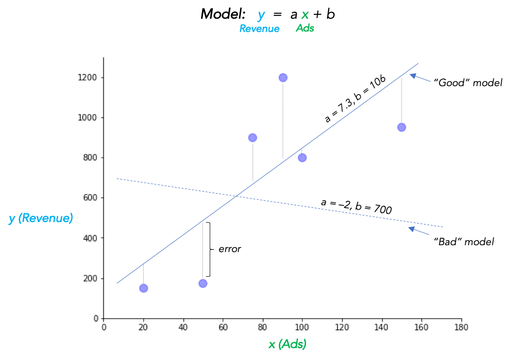
A common way to measure error is with squared error. With the last example, our squared error is $(\text{actual} - \text{prediction})^2 = (175-220)^2$. (Squaring it takes care of negatives, and makes the math easier, although the deeper reason has to do with some of the statistical assumptions connected to this model, which we’ll skip here.)

The average of all our errors over the whole training dataset is called the mean squared error (MSE), which for $a=2, b=120$ is:

\[\begin{align*} \text{MSE} = &\frac{1}{6}\Big((150 - 160)^2 + (175 - 220)^2 + (800 - 320)^2 + \\ &(900 - 270)^2 + (950 - 420)^2 + (1200 - 300)^2\Big) \end{align*}\]

which is a pretty big number.

Now on to minimizing this error. We need to solve the following problem: “Find parameters $a$ and $b$ that minimize the total MSE between the model and the training data.”

One approach would be to just keep guessing different $a$ and $b$, until we get an MSE that is small enough to satisfy us. We could improve this trial and error approach a bit by using common sense as we adjust the parameters, and adjust them in directions that seem to be decreasing the error (for example, if going from $a=2$ to $a=2.5$ seems to decrease the error, we’d probably try $a=2.7$ or $a=3$ next).

Let’s say we use this method and, after lots of napkin math, home in on $a=7.28, b=106.9$ as working really well. In fact, we find adjusting either parameter at all by small amounts seems to increase the MSE. (Feel free to check.) We’re done! So our trained linear model looks like this:

\[y = 7.28 \ x + 106.9\]

Well, almost done: we should worry that although we know $(7.28, 106.9)$ definitely results in smaller MSE than $(7.3, 107)$, what happens with something completely different like $(15.1, 1.7)$? Fortunately, with this linear model we don’t have to worry about this possibility (the term is “global” vs “local” minimums), but it is a very real concern with the more complicated models of the next sections, and we will discuss a few remedies.

This common sense approach of adjusting parameters in a direction with decreases the error, with a little bit of wild trial and error sprinkled in, is the idea behind the actual algorithms modern practitioners use to train state-of-the-art machine learning models, such as gradient descent or its stochastic version. How large of adjustments we’re willing to make is called the learning rate. (The linear model is simple enough we can actually just work out a formula for the optimal parameters, but for most models we won’t have this luxury.)

(Getting-more-technical sidenote: If you remember a little calculus, you m — hey wait, where are you going? — you may recall that to find the minimums and maximums of a function $f(x)$, you can take the derivative, set it equal to zero, $f'(x)=0$, and solve for $x$. We can do the same thing here, with our function being the MSE, and instead of just one variable $x$ to play with, we are fiddling with two: the parameters $a$ and $b$. Gradient means “derivative,” descent indicates we are looking for where the gradient (derivative) is smaller (i.e. close to zero), and stochastic indicates we are inserting some randomness into this process which turns out to sometimes help with big messy models and big messy datasets.)

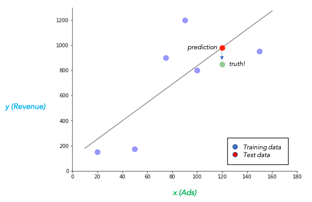
Step 2. Predict

Now comes the real test: we spent $x=\$120$ on advertising this year, and using our model, we predict we will make

\[y=7.28 (120) + 106.9 = \$980.50\]

Unfortunately, when summer’s over, we find we only made $850. Not too far from our model’s prediction, but still kind of a bummer.

Final fitted linear model

Hopefully we kept the limitations of our model in our mind before making any dangerous financial commitments.

Although this particular problem is small enough we’d probably be a lot better off just applying good old-fashioned common sense, for the sake of example let’s start wondering what we can do to improve our model for next year.

So let’s try to expand this framework.

AGI, Specialized AI, and Machine Learning: the big ideas
Peeking under the hood with a linear model
Expanding the framework: bigger data, bigger models
Getting crazy: (Deep) neural networks
A Safari Tour of Modern ML Models
Ethics, Limitations, and the Future of AI

Written on April 2nd , 2020 by Steven Morse