Steven Morse personal website and research notes
4 - Getting crazy: deep neural networks
Series: A (Slightly) Technical Intro to AI
- AGI, Specialized AI, and Machine Learning: the big ideas
- Peeking under the hood with a linear model
- Expanding the framework: bigger data, bigger models
- Getting crazy: (Deep) neural networks
- A Safari Tour of Modern ML Models
- Ethics, Limitations, and the Future of AI
In the first post we gained an understanding of the distinction between specialized AI and the artificial general intelligence (AGI) of our Skynet fantasies, then worked through the big idea behind the most successful and widely applied breed of specialized AI, machine learning (ML). In the second post we worked through the actual mathematics of this idea using a simple linear model, and then expanded this framework a bit.
But when people refer to “ML” and “AI,” they typically don’t have linear regression in mind. In this post, we’ll explore a more modern ML model, the deep neural network, thus the term du jour, deep learning. Then we’ll explore the many variants of this idea (and a few other models too). If you’ve been following along, we’ll see how all these advanced algorithms are extensions of the simple framework we’ve been discussing all along.
(Deep) neural networks
An (artificial) neural network (NN) is a model that takes an input and gives an output, just like our linear model. The details are just a bit more complicated than multiplying by a slope and adding an intercept.
Recall our linear model, which we could think of like this:
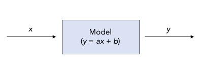
So the model takes in an \(x\) and spits out a \(y\) using the transformation \(y = ax +b\).
Now consider a slightly different diagram:
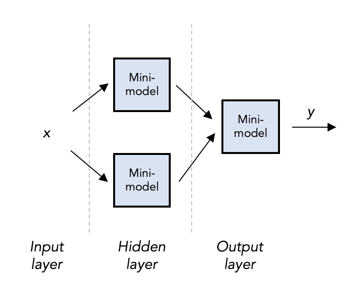
This model qualifies as a (very small) neural network, and we can see it is quite literally a network of small models, each with some inputs and outputs. The “mini-models” are called “nodes” — we refer to the inputs as the input layer, the outputs as the output layer (“layer” since we might want a lot more than one node in each). But the unique part of a NN are the hidden layers, in this example just one hidden layer of 2 nodes. We could have dozens, even thousands of hidden layers, each with thousands of nodes — this is the genesis of the term “deep” neural network.
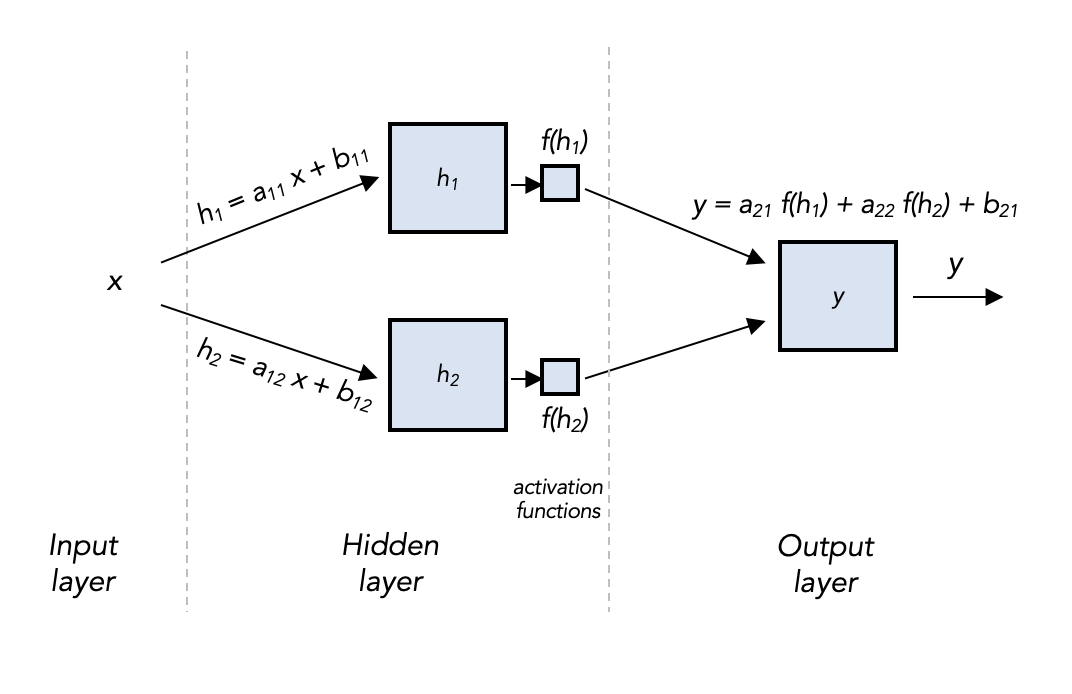
Now for the math. Coming into any hidden layer node, we will apply a linear transformation just like the linear model: starting with the hidden nodes, say \(h_1 = a_{11} x + b_{11}\), and \(h_2 = a_{12} x + b_{12}\). Coming out of any node, we will apply an activation function, for example, \(f(x)=\tanh(x)\), the hyperbolic tangent function. (There are many popular activation functions, which accomplish slightly different modeling effects — here’s a list. Notice though they’re all non-linear: if not, the whole network will simplify to the linear model we had back in Post 2.)
Now coming out of the hidden nodes and activation functions we have \(f(h_1)\) and \(f(h_2)\). Coming into the output layer node, we again apply a linear transformation (now on two numbers), and no activation function, to get \(y=a_{21} f(h_1) + a_{22} f(h_2) + b_2\).
Putting those equations back on the diagram might help:
So really our model still boils down to a single equation, kinda like the linear regression model:
\[y = a_{21} f(a_{11} x + b_{11}) + a_{22} f(a_{12}x + b_{12})\]but writing it like this obscures the network structure (or “architecture”) underneath.
Also, writing it out explicitly gets real tricky when we start to scale this idea up:
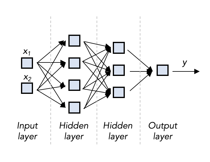
and up, and up:
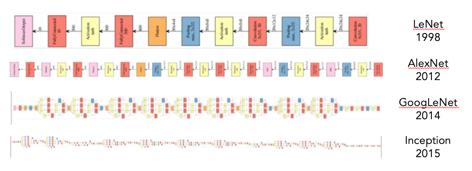
These are the schematics of NNs that surpassed all previous accuracy records for machine image classification, from 1998 to 2015. This is definitely in the realm of so-called “deep” learning. (These were actually convolutional NNs, which we discuss in the next section)
Training a NN
Hopefully, at this point, you’re wondering how you could train such a thing. For the linear model, we only had two parameters to tinker with (slope and intercept), and it seemed reasonable to believe we could choose them in such a way that minimizes error just by doing some random adjustments generally in the direction that made the error get smaller, until we couldn’t get smaller anymore. But our small NN has six parameters, and the large ones have millions!
It turns out, the “random guesses plus small adjustments to reduce error” method still works. As you may recall, this is called stochastic gradient descent, and it is the basis for most common methods for training large NNs.
The tricky part is figuring out how to make adjustments that reduce the error slightly, called backpropagation. With the linear model, we discussed using a little calculus to figure out this adjustment (taking the derivative, setting equal to zero). The same applies here, our function is just a little more complicated and nested. Specifically, an error on the output layer end is the result of dozens, thousands of tiny errors all throughout the hidden layers of the network. We can still take a derivative (“gradient”) and find where it is zero (“descent”), but we note that the change we need on the output layer needs to propagate back through the network for smaller changes deep inside.
So what’s it good for?
What is the point of all this trouble, you may ask. Well, if you recall from the previous post, it is hard to pick the right model in Step 0. If we suppose there is some true model out there that perfectly represents the hidden nature of the process generating the data, how can we find it? One approach we flirted with was picking a model capable of high complexity (like a high degree polynomial), but then brutally punishing it for getting complicated.
Neural networks provide the ultimate solution in this vein. You can show, using some pretty deep math, that a sufficiently large NN can faithfully represent any function. Like, any. So that means no matter how crazy our problem is, if we use a big enough NN, we can perfectly model the underlying function/process and have, essentially, a perfect black box.
A great place to play with these ideas is Google’s Neural Network playground. You can tweak each (hyper)parameter right in your browser and see how the model is able to fit to different datasets. When you press “Play”, you begin the educated guess and check process known as gradient descent. You can literally watch the machine learning. Cool stuff.
Here’s two different NNs trained on the classic “XOR” dataset. The dots are colored by type; the background is colored by how confident the model is where different types should be classified. Ideally the background matches the dots:
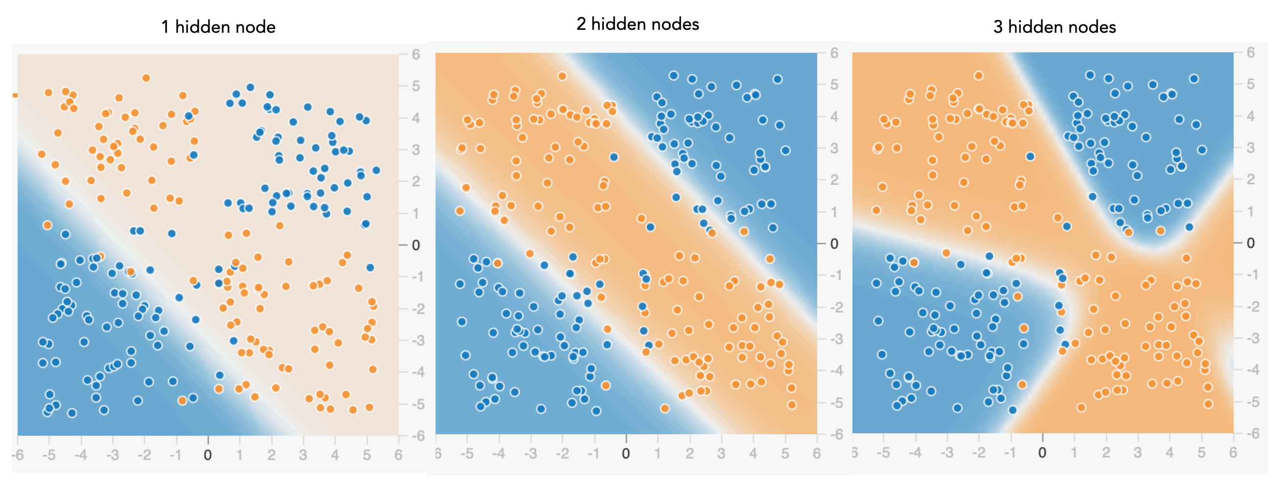
On the left, the NN only had 1 hidden layer with 1 node. Think about that: it’s almost the same as the plain linear regression model, and so it is no surprise it struggles to classify this tricky dataset. As we gradually add hidden nodes to the architecture, the model is able to capture more and more non-linearity.
No free lunch still applies, however: the bigger the NN, the more you risk overfitting and having terrible predictive performance out-of-sample. So we are locked in the same bias-variance tradeoff dance as before, but with a very flexible dancer. You should play with some different datasets, include noise, and see if you can create this overfitting problem: it will show up in some pretty bad test set performance.
Interpretability
A final important topic with deep neural networks (and any complicated ML model) is the challenge of interpretability. Recall with the linear regression, the parameters had nice interpretations: for example, the intercept represented a baseline, the slope represents the importance of the effect of the input. This helps us understand how the model works, which helps us make it better.
Nice interpretations are hard to come by with deep NNs, and it is an open field of research. For example, visualizations of the parameters in a hidden layer may reveal how that hidden layer is transforming the data in a way that assists the model achieve an accurate output — processing facial images, for instance, the first hidden layer may be heavily weighted on areas corresponding to eyes.
But in general, this is very challenging and leads to the anxiety over putting ML models in charge of important decisions, a topic we will revisit in Part 6.
Nothing new under the sun
To close, a quick history lesson is important for context here: neural networks trace their ancestry to 1958 with the invention of the “perceptron algorithm,” originally designed to be a machine that could mimic the structure and function of the human brain. The perceptron stayed out of the AI spotlight, but by the late 1980s, researchers had discovered the major innovations of multiple layers and training through backpropagation. In the 1990s, researchers discovered things like convolutional NNs, recursive NNs, and several critical engineering tricks. But even by the early 2000s, NNs merited very little attention and were not really seen as the future of AI.
It was not until the advent of enormous data availability (“big data”), significant computing advances (most notably, the discovery of repurposing the graphical processing units (GPUs) in a computer’s graphics card to enable massively parallel computation during NN training), and more theoretical innovations, that NNs began to overtake the AI leaderboard.
If you’re interested in going a bit deeper on NNs, I have a couple blog posts here you may enjoy (and there are dozens more elsewhere on the interwebs). Even if you don’t have the necessary multivariable calculus, probability, and coding background, it is worth checking out.
Now let’s explore some important variations on this deep learning theme.
- AGI, Specialized AI, and Machine Learning: the big ideas
- Peeking under the hood with a linear model
- Expanding the framework: bigger data, bigger models
- Getting crazy: (Deep) neural networks
- A Safari Tour of Modern ML Models
- Ethics, Limitations, and the Future of AI