Steven Morse personal website and research notes
3 - Expanding the framework: bigger data, bigger models
Series: A (Slightly) Technical Intro to AI
- AGI, Specialized AI, and Machine Learning: the big ideas
- Peeking under the hood with a linear model
- Expanding the framework: bigger data, bigger models
- Getting crazy: (Deep) neural networks
- A Safari Tour of Modern ML Models
- Ethics, Limitations, and the Future of AI
The straight line framework we explored in Part 2 has, uh, been around a while: Friedrich Gauss invented it (or was it Legendre?) back in 1809. You might hear it called least squares, since we’re minimizing squared error, or linear regression, since it assumes that the data will stay close, or “regress back,” to the line.
But linear regression is an ML model, like it or not, and once you understand it, it’s not too far of a leap to the much sexier models making the news. A mathematical equation or model, selecting parameters based on data using some algorithmic method, predicting on unseen data — all these concepts we saw in the context of a plain line will apply directly to the exotic-seeming models in Part 4 and Part 5.
Before we dive into the deep end, let’s end this post with some ways to extend this framework of the straight line. This will get progressively more technical, but try to hang in to the end.
More data
The first thing we might want is more data. This could mean more observations (like other lawnmowing businesses in the area) or more variables per observation (like weather, or type of advertising).
If we have lots of observations, we could sneak a test run of our predictive ability: for example, instead of training on all the historical data, train on everything except last year. Now last year becomes test data. Do a test prediction by putting last year’s advertising into the model and see how well it predicted last year’s revenue. Later we will expand this idea.
If we have lots of variables, we need a different model:
More variables
More inputs require modifying our model. We notice that not only advertising (\(x_1\)) affects our lawnmowing revenue, but also the amount of rainfall (\(x_2\)). If we still think we should use a linear model, it now looks like this:
\[y = a_1 x_1 + a_2 x_2 + b\]The nice thing is, all our methods from before still apply: we want to minimize squared error over a training set by adjusting our three parameters \((a_1, a_2, b)\), we can use some sort of gradient descent (or in this case, just solve it explicitly), and our ultimate goal is accurate predictions of \(y\).
In fact, we could use as many input variables as we want by extending this framework (we can even predict multiple \(y\) values) … although as our model becomes more complicated, we should have an instinctual concern its increased capacity for capturing the past will inhibit its ability to accurately predict the future. Let’s expand on this topic a little more now.
More complex models
We mentioned we didn’t need to pick a linear model in Step 0. We could’ve picked a polynomial model like this:
\[y = a_4 x^4 + a_3 x^3 + a_2 x^2 + a_1 x + b\]This produces a very curvy curve, whose mesmerizing curviness we can mold by adjusting the parameters \(a_i\) and \(b\).
Let’s use this degree-4 polynomial model to explore two tricky ideas that are critical to machine learning.
Bias-variance tradeoff. Look what happens if we fit the curve to our historical lawnmowing dataset by adjusting \(a_i\) and \(b\) to minimize squared error:
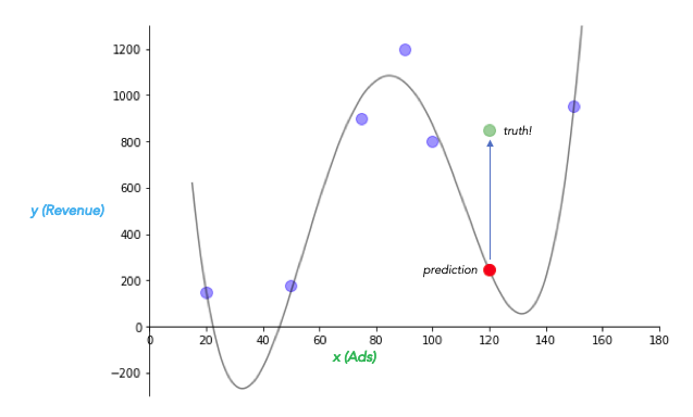
It predicts almost every datapoint in the training set perfectly!
But it does predict negative values, which doesn’t seem right, and it starts producing absolutely massive values for extremely small ad investments. Hmm… And consider that red point, which represents our prediction for this summer. Our model is so closely fitted to the training data, it performs horribly on unseen data! The linear model did a better job. Heck, just picking the average \(y\) value in the historical data would have been a better guess.
This is the “no free lunch” law of statistics and machine learning, called more technically the bias-variance tradeoff. Think of error due to bias as error from overly simple assumptions, and error due to variance as error from being overly sensitive to changes in the data. Our curvy polynomial model has a low error due to bias (almost zero error from model assumptions), but high error due to variance (model does poorly with new data, or a tiny change in existing data). Another way to say this is that it has very low bias, and therefore it is sensitive to variance — it is so flexible it can fit itself to anything, but that means it is easily surprised by new data.
The tradeoff is: as you decrease error due to bias, you always increase variance error, and vice versa.
Another way to think about this is in terms of the training and testing data we discussed earlier: a very unbiased model will do very well on training data, but its sensitivity to variance will make it do poorly on testing data. (Or consider the inverse: a biased model will do pretty poorly on training data, but its insensitivity to variance means, roughly, it will do equally as poorly on testing data.)
We’d like to find the sweet spot. But how?
EDIT: I edited the above section on bias-variance to correct some confusing and inconsistent statements. Thanks to David Touretsky for pointing it out.
Model Selection. So far we’ve described model selection as happening exclusively in Step 0, and it may have felt like a somewhat blind choice. In fact, we can typically combine Steps 0 and 1 a bit and pick our model in a way that ensures it will find the sweet spot of bias-variance tradeoff and generalize optimally in Step 2 (Predict).
The strategy is to choose a very flexible model (think of it as a family of models), and instead of picking parameters by just minimizing squared error, try to also minimize the model complexity.
Our polynomial curvy model is like a family of models. For example, notice that the linear model is contained in the curvy model: just set \(a_4, a_3, a_2 = 0\), and you get:
\[y = 0 \cdot x^4 + 0\cdot x^3 + 0 \cdot x^2 + a_1 x + b = a_1 x + b\]And, the bigger the higher order terms get, the more curvy this curve will get.
So instead of just solving the problem “find parameters that minimize MSE” like before, we might try solving the problem “find parameters that minimize MSE and the size of the parameters,” something like
\[\text{minimize} \Big( \text{MSE} + \lambda\big(\text{size of parameters}\big) \Big)\]This fairly straightforward intuition is called regularization, and it’s the idea behind how we can use the extremely complicated models in the next section without the overfitting problem.
This brings us back to finding the sweet spot: we need to specify how much we care about model complexity, that is, we need to specify the tradeoff parameter \(\lambda\). (This is actually called a hyperparameter, since it’s part of our meta-problem of model selection, not a parameter like the slope or intercept.) One way to do this is by taking our training data and carving off a piece to use as a validation set (or “hold out set”). Then we do a little dance: pick a value for \(\lambda\), train the model on the training data, test it on the validation set, then pick a new value for \(\lambda\) and repeat. Look at all your performances on the validation set, and pick the \(\lambda\) that did the best. The thought is (and this can be made mathematically rigorous) that this model will also do the best on new, unseen test data, so long as that test data looks reasonably similar to the training and validation data.
Curse of dimensionality. As we scale up the complexity of our data and models, it is wise to keep a certain specter in mind known as the curse of dimensionality. We have so far been dealing with one input variable (\(x\)), and been able to depict our models in 2-dimensions. As we’ve already mentioned however, we’d like to use many more input variables.
As we scale up the dimensionality of our problem, it becomes increasingly difficult to accurately capture dependencies in the data, measure error, much less maintain any intuition about what’s going on. A cooler superpower than flying, I submit, is an ability to visualize high-dimensional spaces.
One common example will give you a sense of the strange challenge higher dimensions pose. Picture a circle drawn inside a square, so it touches the edges. The circle’s area is almost as big as the square’s, right? Now go up a dimension, to a sphere inside a cube. There seems to be a little more space in those corners, but the sphere is still taking up most of the interior volume. Now go up another dimension, which no longer makes sense visually, but we can represent perfectly well with mathematics: now we have a hypersphere inside a hypercube. It turns out as the dimension goes from 4, to 5, to 100, the hypersphere’s volume is only a tiny fraction of the enclosing hypercube’s, even though it is still touching on the edges. This is absolutely astounding. And when we measure distance between two points (like error), this distance becomes vanishingly small compared to the enclosing space as we go to higher dimensions, so things like minimizing error become increasingly finicky.
Classification
Ok — we’ve covered an enormous amount of challenging material in this post. Let’s end with something a little easier to grasp.
Our running example of the lawnmower business had a number as input and a number as output — moreover, those numbers were continuous, meaning we allowed any sort of dollar amount, $40.25, even $13.111578, etc.
Often we want to construct models that have discrete inputs and/or outputs. Our cat/dog image classifier from the first post is an example of a model with continuous inputs (the values of the pixels of the image) but discrete outputs (“cat” or “dog”). Problems like this with discrete outputs are often termed classification problems, whereas problems with continuous outputs are often termed regression problems.
The figure below depicts some data that comes in two types, X’s and O’s, plotted according to two arbitrary measurable variables we know about each datapoint (say, height and weight for men and women). A classifier model could be something as simple as a straight line that does a good job of separating the two types. We can also devise ways to express the probability that our model’s prediction is correct, based on “how far” it is from the line, subject to several assumptions about the data.
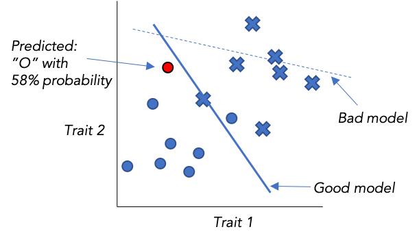
You should not be surprised now that like linear regression, this idea of a linear classifier is nothing new, but is the basis for the powerful new, and highly non-linear methods of the next section. You should also correctly guess that to train such a model (i.e. find the best line) involves essentially the same process as with our least squares model.
As a more concrete example, consider training a ML classifier model to take patients’ chest X-rays and predict whether they have cancer. Or consider how your email app knows to classify certain emails as “Spam” just based on their content — the use of machine learning for spam detection is almost as old as email itself. We’ll encounter many more examples as we go.
In the next posts, we’ll extend all these ideas to neural networks and then take a safari ride through the current field of commonly used ML models. Our intuitions from this section on a simple linear regression model will, hopefully, extend to the more exotic models.
On to Part 4!
- AGI, Specialized AI, and Machine Learning: the big ideas
- Peeking under the hood with a linear model
- Expanding the framework: bigger data, bigger models
- Getting crazy: (Deep) neural networks
- A Safari Tour of Modern ML Models
- Ethics, Limitations, and the Future of AI