Steven Morse personal website and research notes
5 - Safari Tour of Modern ML Models
Series: A (Slightly) Technical Intro to AI
- AGI, Specialized AI, and Machine Learning: the big ideas
- Peeking under the hood with a linear model
- Expanding the framework: bigger data, bigger models
- Getting crazy: (Deep) neural networks
- A Safari Tour of Modern ML Models
- Ethics, Limitations, and the Future of AI
The power we now possess with deep neural networks opens many doors. We’ll explore several important variations on this theme — convolutional NNs, recurrent NNs, GANs, reinforcement learning — that each structure the neural network to take advantage of some inherent aspect of the data or problem at hand. For good measure, we’ll also take a look at some other popular and important, but non-deep-learning, ML models.
Deep learning rules everything around me
Convolutional neural nets
Convolutional neural networks (CNNs) take advantage of the fact that within a single observation in the data, there may be some inherent structure. For example, the position of facial features in facial images.
Using our cat/dog image classification example, and with the rough outline of how an actual NN works in your mind, consider what the structure of a NN classifier should look like. The input layer is an image — square, perhaps, like \(n\times n\) pixels. The output is two values: probability of image being a dog and probability it is a cat.
It turns out to be helpful to gradually winnow down the large input layer through successively smaller hidden layers — this helps us keep track of that inherent structure. For example, in the first hidden layer, have each node aggregate the input from, say, a 4-pixel subsquare. If the input images are \(32\times 32=1,024\) nodes, the first hidden layer would only need 64 nodes. We could continue this condensing of the input layer all the way to the output layer. (Actually, we typically allow some overlap in the subsquare patches, and we don’t use the same size patch in each hidden layer, and images are more often input with a third dimension representing depth or color, but you get the idea.) This act of combining and pooling information is known as convolution, thus the name.
This all gives a network architecture something like this:
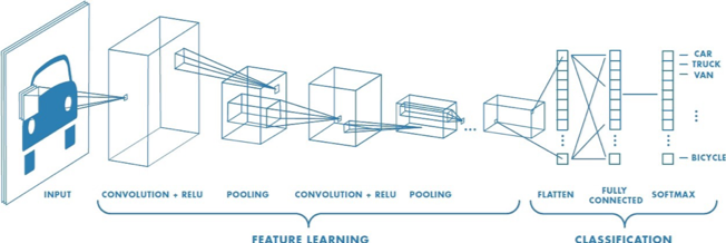
Interestingly, we usually observe each hidden layer starting to specialize in different aspects of the image recognition task: the first layer might discriminate what part of the image is the face vs. the background, while the second layer discriminates facial features, etc. And magically, this happens simply by setting up the network structure (i.e. the mathematical model), giving it some training data, and executing a parameter estimation technique like stochastic gradient descent.
If you recall our discussion about model complexity and regularization, notice that by forcing a more restrictive structure on our CNN, we’ve automatically decreased the model complexity in a purposeful way from the naively fully connected NNs in the previous post.
Recurrent neural nets
CNNs are designed for input data where each observation has inherent internal structure. What if successive observations have inherent relationships, like prices over time, or words in a sentence? This leads us to recurrent neural networks (RNNs).
The big structural idea of an RNN is that each layer passes its values not just forward into the next layer like before, but also backward into previous layers. This allows the network to retain a sort of memory of past events.
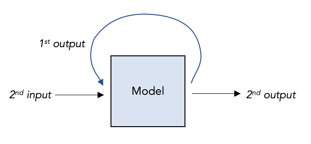
As you might expect, RNNs get applied in many settings with an underlying time sequence (“time series data”), like stock forecasting (although nota bene I am not recommending this). They’re also very successful in natural language processing (NLP): after all, is a sentence anything more than a sequence of words (inputs), each of which shares inherent relationships with its predecessors? What comes next in this sentence: “I live in India. I speak _____.” To accurately predict the blank, a model needs a short-term memory to recall the word “India” that came earlier in the phrase, and a long-term memory to recall that likely fill might be “Hindi.”
Consider this little experiment: we could give the RNN a word, have it predict the next word, feed that word back into the RNN, and repeat … generating entire passages. Here’s an example of doing this with an RNN that was trained on the works of Shakespeare:
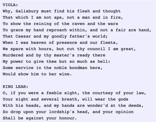
What’s even more amazing about the above example is the network was generating the passage not word by word, but letter by letter.
Generative Adversarial Networks (GANs)
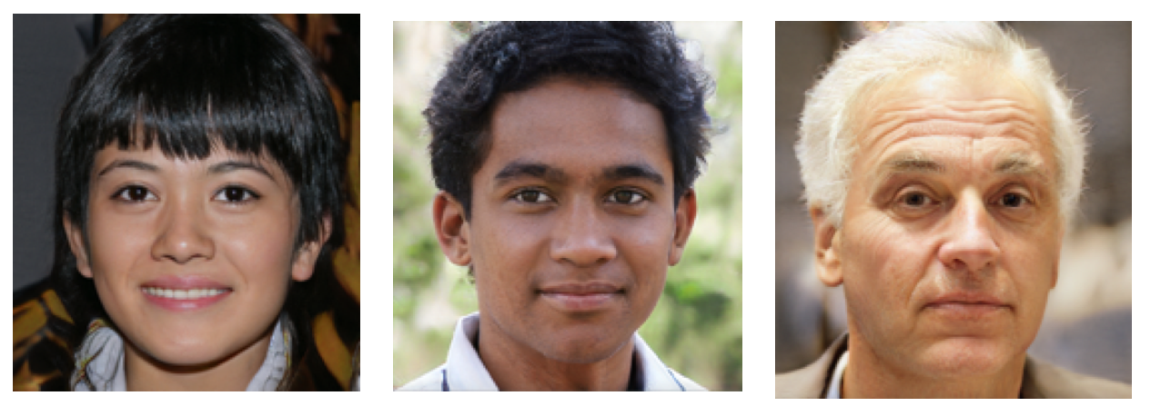
One of the most mesmerizing innovations of NNs to me are Generative Adversarial Networks, or GANs. Here’s an example of the idea: design NN #1 to take some generic image input and output a convincing, more detailed variation on that image. Then design NN #2 to take an image and classify it as real or fake. Finally, use the feedback of NN #2 to improve the faking ability of NN #1, and vice versa. You have now placed two powerful ML algorithms in mortal combat to out-optimize each other, and the results can be terrifying.
A fairly benign application of this innovation is to allow computers to generate convincing images or videos for gaming, backgrounds, etc. Here are three faces generated by a GAN, and do not represent the faces of real people. Pretty convincing.
A more (potentially) nefarious application is to have computers generate convincing false video, for example, of a state leader denouncing a neighbor government — these are termed “deep fakes.” (And now you know what “deep” really means!) Here’s a video of a GAN superimposing a person’s face on an actor in real time.
Reinforcement learning (RL)
Reinforcement learning (RL) traces its origins to the 1950s, and it is a different animal than the models we’ve discussed so far: it’s not really supervised, since we will give RL models inputs but only occasionally give it outputs (so we say “semi-supervised”), and it’s not inherently NN-based, although we’ll see its modern popularity has grown after infusing it with NNs. RL has recently beat the world grandmaster at Go, it has self-taught simulations how to walk, it is at the heart of the algorithms which control autonomous vehicles, and seems to be making inroads in stock trading.
RL is the idea that we can take a (computer) agent, allow it to take actions in some state where it receives rewards for certain actions, and over time, it will learn to act nearly optimally. This means we don’t need petabytes of data anymore, we just need to be able to enforce the rules of an environment and allow the agent enough time to explore and learn in that environment.
For flavor, let’s try to wrap our heads around a common brand of RL called Q-learning. Imagine you are a computer trying to learn to play chess. For any given board position, you have a few dozen options of possible moves. You have no idea which move is better than any other, so you just play randomly and lose a lot of games. Each time you lose, you go back along the trail of decisions that got you there and mark them as bad, being less pessimistic the further back you go, since your first few moves contributed less to your loss than your final moves, and are therefore less bad. Finally, you win a few games, and update those trails as good. You might even allow some intermediate rewarding of actions if nice things happen like capturing the queen or setting up a really juicy fork. (This is the idea behind dynamic programming and more specifically, Bellman’s equation, the essential piece of math that makes RL work.)
You are a computer, so you work at this tirelessly for several million games. You record your lessons learned in a table, called a Q table: on the left, all the millions of board positions you have encountered, along on the top, all the possible actions one may take in chess, and in each cell, the “goodness” of that action from that position in terms of the final reward (win/lose). We call this “goodness” a q-value. If we play enough games (our training step), these values will allow us to make pretty good decisions and win games (our predict step).
But …. chess is too complicated to try listing all possible moves and board positions, much less train on all of them. This limitation of Q-learning kept it mostly on the shelf, despite its discovery in 1989.
Enter Google’s DeepMind research laboratory, which in 2013 applied deep neural networks to Q-learning and started turning heads. First it learned to play Atari at human levels, and later it was a piece of the AlphaGo algorithm that defeated Lee Sedol at Go.
Remember our Q table? Think of it as a function, or black box: input a state and an action, output a q-value. As we know, neural networks are very good at representing very complex functions. DeepMind’s insight was to do Q-learning, but train a deep NN to mimic the Q-table along the way, so that when training is complete, even though you haven’t seen a certain state-action pair, your NN can give you an approximate value for it. Just like our linear model in Part 2 had never seen our ad spending for the upcoming summer, it could provide a prediction.
RL is a huge, active field, and deep Q-learning is just one variant, and it has broad, powerful applications as mentioned earlier. RL is also perhaps the most compelling of the algorithms we’ve explored because it seems so humanlike. AlphaZero has learned to beat its predecessor by training purely onself-play. Recently, DeepMind used RL to propose a new understanding of the reward mechanisms of our brain. One might even trace RL’s heritage back to experiments in the 1950s to replicate animal learning with computers. Often, when people begin breathlessly speculating about the future potential of AI, a deep-RL algorithm has made a recent impression on their mind.
Other Hall of Famers
Not all of what you hear about in modern ML falls in the category of deep learning, however. Let’s try to get the flavor of a few other popular models.
Ensemble learning
Random forests
Imagine you are trying to develop a classification model to help decide what applicants to hire for your company, based on historical data of successful hires. This has some tricky ethical considerations we’ll discuss later, but for now, consider the simplest possible classification model: take their work experience, and if it’s more than 5 years, hire them, if not, don’t. Based on this single decision, you could examine past data and assign some sort of accuracy score to this model, like what percentage of people with more than 5 years experience were successful hires. You could extend this idea and come up with additional criteria: what level education do they have, and so on. This type of model is called a decision tree, and unsurprisingly, we can have a machine learn what these questions and thresholds should be to optimize the accuracy, just as with all our previous models.
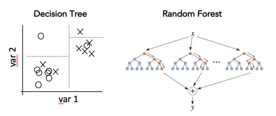
Instead of just one decision tree, with large and complex data it is often better to create many, many decision trees, each focused on a random different subset of input variables, and then average their outputs. This is called a random forest (get it? lots of trees make a forest??). The technique of re-using parts of a dataset in different ways is called bootstrapping, and the averaging at the end is called aggregating, so random forests are a type of ensemble learning called bootstrap aggregating, or “bagging.”
Like NNs however, the cost of increasing accuracy from a decision tree to a random forest is a loss in interpretability.
Boosted methods
Another type of ensemble learning is boosting. The idea here is to train a sequence of small decision trees, and in each one, focus on the part of the dataset which the previous trees had the hardest time accurately classifying. Although this method can be sensitive to outliers, it is generally considered one of the strongest “out of the box” models, requiring very little experienced tweaking to get top-shelf results.
Bayesian methods
Lumping all of “Bayesian methods” into a subsection is a bit disingenuous, since there are Bayesian versions of nearly every model we’ve discussed so far, so in a sense Bayes has been with us all along.
Bayes’ theorem, named after the Reverend Thomas Bayes, says that if you start off believing a coin is fair, but then you observe a few dozen heads flipped in a row, you no longer believe it’s very fair. Well, his theorem says this in a much more general, probabilistic way, but the idea is: we have some prior belief about the probability of a certain hypothesis \(H\), we have some likelihood of some event (or evidence) \(E\) happening given that prior, and we have the posterior probability of \(H\) being true after having observed \(E\). In the language of probability,
\[P(H|E) \propto P(E|H)\cdot P(H)\]where the notation \(P(H\vert E)\) reads “probability of \(H\) given \(E\)” and the little \(\propto\) means “proportional to.”
(Notice we started talking about “belief”. I thought this was math! There is a whole tribal rivalry between so-called “Bayesians” and “frequentists” that leads to different interpretations of Bayes’ theorem and the implications it has on statistics and life itself. It is fundamentally important to everything we’ve been discussing, and so naturally I will completely bypass here.)
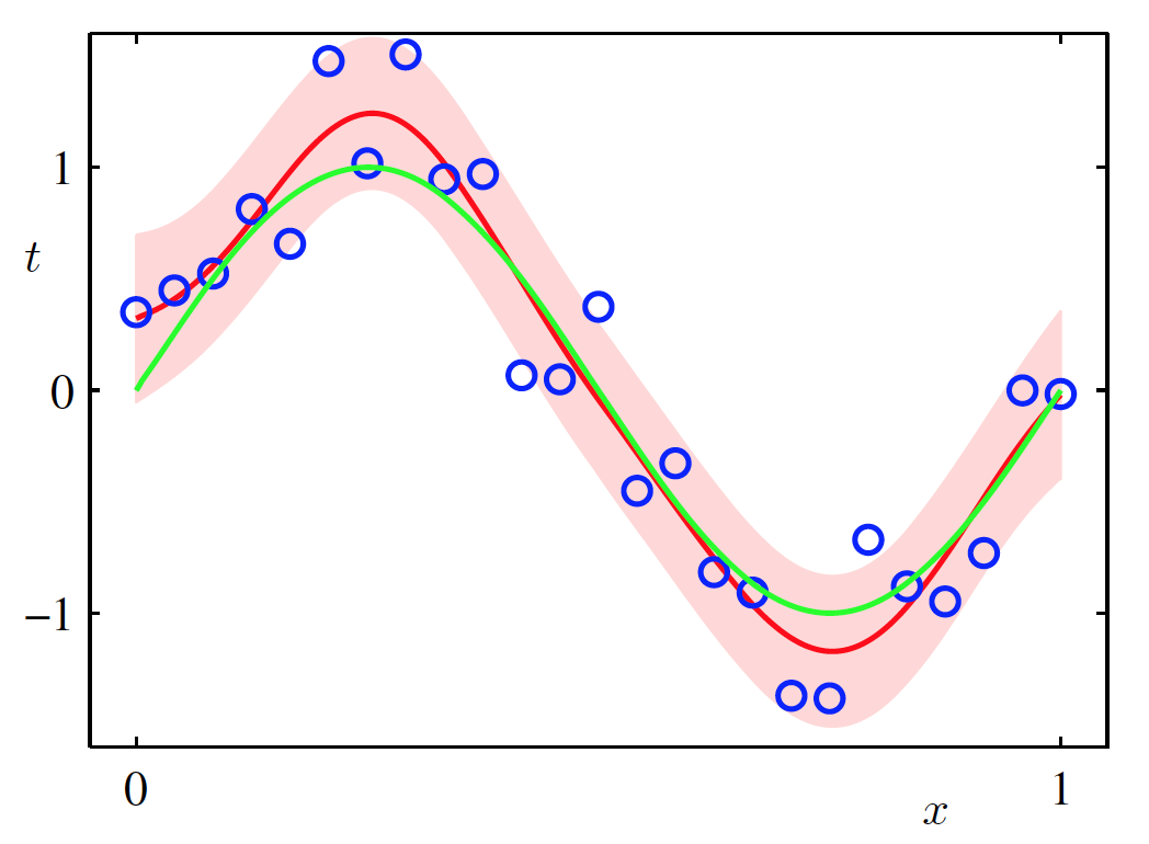
Anyway, one big idea in Bayesian approaches is to incorporate a prior belief in your model: in our linear model, we just let our parameter values be whatever they wanted, but in a Bayesian approach we would specify in advance that we would much prefer the coefficients on the large degree terms to be quite small. This is the Bayesian way of regularizing model complexity, and in many cases, certain priors lead to identical results as the non-Bayesian approach.
Another big idea in Bayesian approaches is to never discard information as you’re building and training and testing a model. Specifically, you specify a probability distribution for any unknown value, like a parameter, which describes how likely different values are (the classic “bell curve” is a type of probability distribution). Your prior, your posterior, all need distributions, and the posterior’s gets “updated” as you examine more data (what we have been referring to as “training”). Instead of your final model being a single line, your final model is a distribution of possible lines, weighted by which ones suit the data better. And if you need your prediction to be, like, a single number so you can actually take an action, Bayesians say, ok fine, if you must, use the mean (average) of the distribution.
Unfortunately, these ideas, while beautiful, lead to extremely difficult calculations when we apply them to Reverend Bayes’ little theorem. As a result, Bayesian approaches usually involve lots of heavy computations and simulations — techniques like Gibbs sampling, or Markov chain Monte carlo (MCMC), or variational inference.
Bayesian approaches tend to have better performance in many applications, and are often less used only because of these mathematical and computational challenges, not any philosophical prejudices. (As an aside, a non-philosophical objection I have read to Bayesianism is that it relies on well-behaved distributions so that the posterior will converge to something meaningful after a reasonable amount of evidence/data — this is fine for well-behaved things like language processing, but a flawed assumption when extremal events are more likely, like the stock market.)
Dimension reduction
Most datasets are high dimensional, that is, many variables for each datapoint. A hundred years ago, a dataset of human measurements would probably contain height and weight for each person. Now, a laser scan could provide us hundreds of measurements per person, from upper torso length to circumference of right wrist. Although, there won’t be much difference between the “right leg length” and “left leg length” values, do we really lose much by replacing both with an average, and reducing the dimension of our problem by one?
There are principled ways to approach this dimension reduction problem. Possibly the best way is low-tech: use domain expertise to manually select or create a better set of features out of the available raw data. But there are automated ways as well: the averaging approach is a simplistic version of a family of techniques that project the dataset down into a lower dimensional subspace (think of the projection like a 2-D shadow of a 3-D object).
For example, principal component analysis is a technique from classic statistics that finds a flatter representation of a dataset which maximizes the amount of variation still explained by the smaller dataset.
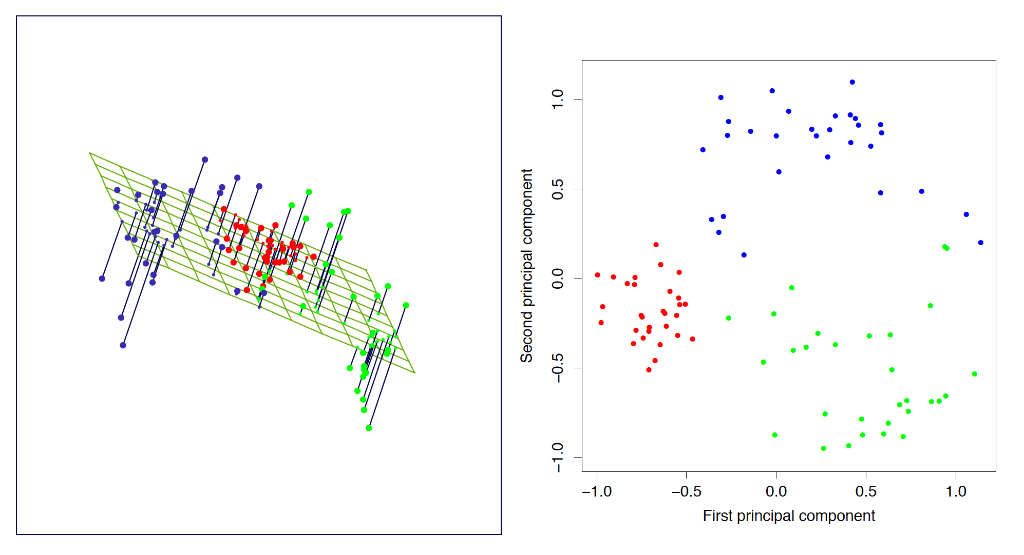
In the image above (taken from Elements of Statistical Learning), a set of points in 3-D (left) is projected onto a plane, resulting in new coordinates in 2-D (right).
More recent methods take different approaches: for example, t-SNE tries to find a low-dimension representation of the data such that, roughly, if two points are similar (close) in the original dataset, they are likely to be close in the smaller one.
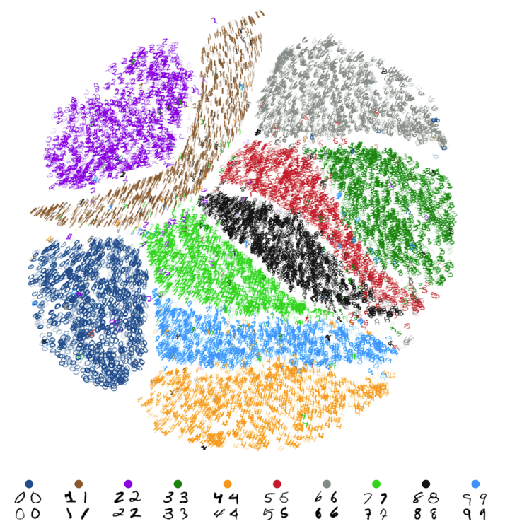
In the image above (credit: Nicola Pezzotti), t-SNE is applied to a high-dimensional dataset consisting of images of handwritten digits (the famous MNIST dataset). In the resulting low (2) dimensional image, the digits naturally separate into homogeneous groupings, which are colored to demonstrate the stark groupings. The somewhat magical part is that t-SNE produces this without access to the image labels, only the raw images themselves.
Clustering
This brings us to the final category of ML models we’ll get familiar with: clustering methods. The essential idea is to group a set of datapoints in such a way that datapoints in the same group (or “cluster”) are more similar to each other than datapoints in other clusters. Similar to dimension reduction, this is an unsupervised learning task because we are not associating the data with any sort of label or target value — in fact, we want to discover the labels ourselves, through some intrinsic pattern that we believe is hiding in the data.
There are two essential tasks here: first, define what “similar” means and second, figure out a way to find a good grouping of objects without exhaustively trying every possible combination. One example of a similarity measure is the squared difference that we were using to measure error in the least squares model (this is called the Euclidean distance). One example of finding good groupings is to start by finding all the closest pairs, then pair those pairs, etc., and stop joining groups together when the distances become unreasonably big, whatever that means for you (this is called hierarchical clustering).
Applications of this idea abound: market research (finding groupings in a customer base, or finding customers with similar tastes to make product recommendations), bioinformatics (automating genotyping), social networks (finding social network structure), image segmentation (like border detection), and on and on.
Here’s a playful clustering I did a couple years ago of NFL wide receivers based on similar distributions of yardage gains.
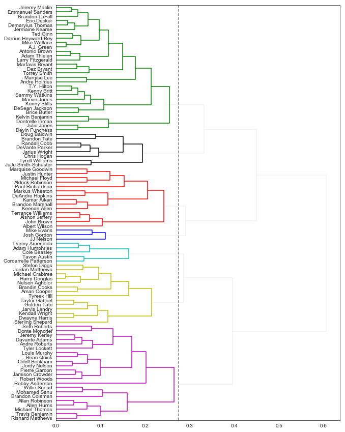
Notice how “explosive players” like Randall Cobb and Doug Baldwin get grouped together, while players used more for checkdown plays like Tavon Austin or Cole Beasley get a different group. (I know, it’s ridiculous.)
Okay, you’ve made it through all the technical bits of this series, let’s close with some nice, non-technical pontificating about the limitations of ML and where the experts think the future lies.
- AGI, Specialized AI, and Machine Learning: the big ideas
- Peeking under the hood with a linear model
- Expanding the framework: bigger data, bigger models
- Getting crazy: (Deep) neural networks
- A Safari Tour of Modern ML Models
- Ethics, Limitations, and the Future of AI