Clustering NFL Wide Receivers by Individual Play Distributions

Written on August 19th, 2018 by Steven Morse

I saw a tweet by one of the Football Outsiders guys poking some fun at Dak Prescott for a quote about Cole Beasley. Here’s the quote:

Dak Prescott on @nflnetwork asked about his go-to receiver: "It's Cole Beasley. ... He can stretch the defense, so it's about moving him around, making the defense respect that he can beat you over the top. Once we open that up, he's hard to cover underneath. That's his game."
— Jon Machota (@jonmachota) August 8, 2018

and here’s the tweet:

57% of Beasley's career catches have gained less than 10 yards. 82% of have gained less than 15 yards. https://t.co/M0T1wzIHyn
— Vincent Verhei (@FO_VVerhei) August 8, 2018

So I think he’s implying with these two stats: Cole Beasley is not a deep threat because the large majority of his plays are short to medium. And therefore it is ridiculous to say defenses are scared of him.

Picking these two stats to make this implication felt wrong to me. I replied with my thoughts, and he graciously humored me, but I totally botched communicating my point and … oh well. Let me try again here:

If 82% of your plays are for under 15 yards, but the other 18% are all for 40+ yards, then you are certainly a “deep threat,” and you would certainly scare defenses! Whether that’s the case for ol’ Cole is irrelevant: the stat doesn’t show what I think Verhei’s trying to show.

Perhaps Verhei’s assumption is: a player who gets 80% short yardage and 20% all-time highlight reel, does not exist in the NFL. (More likely it’s not his assumption, he knows it’s true because he’s a professional football analytics guy and he’s been staring at these numbers for decades.)

I think this assumption is probably right, but I’d like to check, and I’d also like to offer a little more thorough (but still intuitive and non-technical) way of characterizing a receiver.

Spoiler: Cole Beasley’s other 18% of yardage is pretty league-average, is not secretly amazing, and is most similar to players like Danny Amendola and Cordarelle Patterson in terms of catch yardage rates.

Teaser: 77% of another receiver’s career catches were also under 15 yards. But 15% of his catches were for 35+ yards. Can you guess who?

Disclaimer: I’m not a Cowboys or Cole Beasley fanboi. Just a nerd chasing a question. Go Hawks!

The plan.

Scrape individual play outcomes for all active wide receivers from Pro Football Reference.
Check: are there players with mostly short plays but a considerable rate (say, >10%) of “huge” plays.
Cluster similar players based on their entire distribution of catch yardage rates (i.e. use smaller bins than “small-medium-long”).

The Data

The data is easy enough to come by because of the awesomeness of Pro Football Reference. Here’s an earlier post I did on pulling this kind of data in R. For this post I’ll do it in Python. We’re interested in wide receivers, so let’s grab the list and the associated PFR link to all WRs, ever:

# grab wrindex table
r = requests.get('https://www.pro-football-reference.com/players/wrindex.htm')
soup = BeautifulSoup(r.content, 'html.parser')
parsed_table = soup.find_all('table')[0]  

# save as DataFrame (can't use read_html bc want to grab URL)
data = []
for row in parsed_table.find_all('tr')[1:]:
    # first entry is <th>, others are <td>
    th = row.find('th')
    data.append([th.a.get_text(), th.a.get('href')])
    data[-1].extend([''.join(td.stripped_strings) for td in row.find_all('td')])
df = pd.DataFrame(data, columns=['Name', 'URL', 'Pos', 'AV', 'StartYear', 'EndYear'])

# convert numeric columns to numeric
df = (df
 .assign(AV = pd.to_numeric(df['AV']),
         StartYear = pd.to_numeric(df['StartYear']),
         EndYear = pd.to_numeric(df['EndYear'])))

Now, we can loop through each name, access their receiving plays page (by season), and save what we want to a pandas.DataFrame.

cols = ['Tm', 'Opp', 'Quarter', 'ToGo', 'Yds', 'EPB', 'EPA', 'Diff']
wrs = pd.DataFrame(columns=cols + ['Year', 'Name'])
for ix, row in df.query('EndYear == 2017 & Pos == "WR" & AV >= 10').iterrows():
    print(row['Name'], '...', end=' ')
    for yr in range(row['StartYear'], row['EndYear']+1):
        print(yr, end=' ')

        # grab individual plays table
        stem = row['URL'][:-4]  # grab player url stem
        r = requests.get('https://www.pro-football-reference.com' + stem + '/receiving-plays/%d/' % yr)
        soup = BeautifulSoup(r.content, 'html.parser')
        try:  # some players have no plays (should be filtered out with AV >= 10 tho)
            table = soup.find_all('table', id='all_plays')[0]
        except IndexError:
            continue

        # convert to dataframe and add to wrs df
        plays = pd.read_html(str(table), flavor='bs4')[0]
        plays = (plays
         .filter(cols)
         .assign(Year = yr, Name = row['Name']))
        wrs = wrs.append(plays, sort=True)
    print()

Larry Fitzgerald ... 2004 2005 2006 2007 2008 2009 2010 2011 2012 2013 2014 2015 2016 2017 
Brandon Marshall ... 2006 2007 2008 2009 2010 2011 2012 2013 2014 2015 2016 2017 
Antonio Brown ... 2010 2011 2012 2013 2014 2015 2016 2017 
Julio Jones ... 2011 2012 2013 2014 2015 2016 2017 
DeSean Jackson ... 2008 2009 2010 2011 2012 2013 2014 2015 2016 2017
...

I’m filtering by PFR’s AV stat. This takes quite a while, so I saved to a CSV at the end.

Catch yardage

Getting the career rates by yardage

Now let’s look at the field of WRs from the perspective of their career individual play yardage rates.

Here’s some Python-fu to grab only completions, bin by 5-yd windows (a bit arbitrary but seems standard enough), and turn it into a percentage.

# make a completions-only dataset  (Completions are NaN's in df)
z = (wrs
 .dropna(axis=0))

# compute plays by category
z = (z
 .assign(cat = pd.cut(wrs['Yds'], 
                      bins=[-100,-1,4,9,14,19,24,29,34,39,44,49,100],
                      labels=['<0', '0-4', '5-9', '10-14', '15-19', '20-24', '25-29', 
                              '30-34', '35-39', '40-44', '45-49', '50+']))
 .groupby(['Name', 'cat'])
 .agg('size')
 .reset_index())

z.columns = ['Name', 'cat', 'n']
z['n'] = pd.to_numeric(z['n'])

z = (z
 .pivot(index='Name', columns='cat', values='n')
 .fillna(0))

# get rid of categorical index
z.columns = z.columns.categories

# create column of total
tot = np.sum(z, axis=1)

# divide each column by total catches
z = z.div(tot, axis=0)

z['Total'] = tot

# make name a column
z = z.reset_index()

z.head(5)

	Name		<0			0-4			5-9			10-14		15-19		20-24		25-29		30-34		35-39		40-44		45-49		50+			Total
A.J. Green		0.010870	0.108696	0.304348	0.239130	0.144928	0.072464	0.021739	0.010870	0.016304	0.019928	0.010870	0.039855	552.0
Adam Humphries	0.013699	0.157534	0.397260	0.239726	0.102740	0.013699	0.034247	0.006849	0.013699	0.020548	0.000000	0.000000	146.0
Adam Thielen	0.016484	0.120879	0.291209	0.208791	0.148352	0.093407	0.038462	0.016484	0.021978	0.016484	0.010989	0.016484	182.0
Albert Wilson	0.041667	0.150000	0.250000	0.283333	0.125000	0.050000	0.025000	0.008333	0.016667	0.033333	0.008333	0.008333	120.0
Aldrick Robinson0.000000	0.058824	0.235294	0.308824	0.132353	0.073529	0.044118	0.029412	0.014706	0.014706	0.044118	0.044118	68.0

Let’s check on Cole:

	Name		<0			0-4		5-9			10-14		15-19		20-24		25-29		30-34		35-39	40-44	45-49		50+			Total
20	Cole Beasley	0.003984	0.14741	0.418327	0.250996	0.091633	0.055777	0.011952	0.007968	0.0		0.0		0.007968	0.003984	251.0

There’s the 55% under 10 yds and 82% under 15 yds, as claimed (although pretty sure you can get this straight from PFR’s search system, no Python required).

Viz

Now my hypothesis was: just telling us that 82% of a receiver’s catches are under 15 yards doesn’t tell us what the other 18% are, and if that 18% are all huge plays, then we’re looking at a good receiver. Now let’s plot each active receiver with their 0-14 yd rate on the y-axis, and their 40+ yd rate on the x-axis. We’ll size the dots by how many total career catches the receiver has. (I’ll spare you the tedious matplotlib code…)

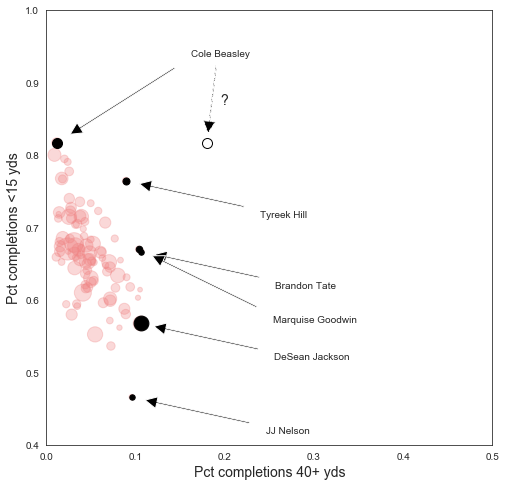
I’ve been cheeky and made a little circle representing a Theoretical Beasley: that is, a Cole Beasley who is theoretically possible given only the knowledge that 82% of his plays are under 15 yds. This Theoretical Beasley, you’ll note, is an extreme outlier and would obviously terrify defenses despite his pedestrian 82% rate of <15 yd catches.

But players like Theoretical Beasley don’t actually exist. Some of the more extreme outlier players are labeled, but overall its a clear linear trend. Beasley’s actual company up there is:

(z
 .assign(a15 = np.sum(z[['0-4', '5-9', '10-14']], axis=1),
         a40 = np.sum(z[['40-44', '45-49', '50+']], axis=1))
 .query('a15 > 0.75 & a40 < 0.05')
 .filter(['Name', 'a15', 'a40', 'Total']))

	Name				a15			a40			Total
Adam Humphries			0.794521	0.020548	146.0
Cole Beasley			0.816733	0.011952	251.0
Cordarrelle Patterson	   0.766871	0.018405	163.0
Danny Amendola			0.800000	0.009412	425.0
Jarvis Landry			0.767500	0.017500	400.0
Sterling Shepard		0.790323	0.024194	124.0
Tavon Austin			0.777202	0.025907	193.0

That feels about right.

Clustering by catch yardage distributions

Instead of looking at two arbitrarily selected bins, like <15 and 40+, let’s look at their entire empirical distribution of catches by yardage (i.e. histogram), and try to group similar players together based on these distributions (histograms). This still requires us to make a choice on bins, but we can chop it up a lot more finely.

There are many approaches to clustering probability distributions. One is to treat the histogram as a vector. The advantage here is simplicity and the wealth of clustering algorithms for Euclidean metric spaces; disadvantages include the challenges with choosing the “right” bin widths, and treating different parts of the distribution the same. Another approach is to fit a parameterized distribution and cluster in the parameter space; advantage here is we still have a lot of clustering options and are less worried about binning; disadvantage is we have to choose a distributional form for our entire dataset, or get a bit fancy with kernel density estimators (perhaps another post?). Still another is the so-called earthmover distance which measures how much probability mass you’d have to move to make one distribution into another — the lower the number, the closer the distributions must be — disadvantage here is we have to solve a small linear optimization problem just to get the similarity measure between two distributions.

Since this is a blog, I’ll stick with the histogram-vector approach, which allows us to represent each WR as a vector in “catch yardage rate space”. We can then apply our favorite clustering algorithm to group similar vectors together.

I’m going to use hierarchical clustering, because it gives me an opportunity to share a little trick for overcoming some inadequacies of the sklearn implementation.

Let’s import:

from sklearn.cluster import AgglomerativeClustering
from scipy.cluster import hierarchy

The catch with sklearn’s agglomerative clustering class is that it doesn’t provide a built-in record of intra-cluster tightness, much less a convenient way to plot a dendrogram of the results. The scipy package has a hierarchical clustering method with this and other functionality (here’s a really nice post), but let’s say we’re stubborn and want to use sklearn!

Fortunately, somebody on stack overflow already solved this problem for us (actually there’s a couple remedies out there), here’s the important method copied nearly verbatim from the SO post:

def get_distances(X, model, mode='l2'):
    distances, weights = [], []
    distCache, weightCache = {}, {}
    for childs in model.children_:
        c1 = X[childs[0]].reshape((X.shape[1],1))
        c2 = X[childs[1]].reshape((X.shape[1],1))
        c1Dist = 0
        c1W = 1
        c2Dist = 0
        c2W = 1
        if childs[0] in distCache.keys():
            c1Dist = distCache[childs[0]]
            c1W = weightCache[childs[0]]
        if childs[1] in distCache.keys():
            c2Dist = distCache[childs[1]]
            c2W = weightCache[childs[1]]
        d = np.linalg.norm(c1-c2)
        cc = ((c1W*c1)+(c2W*c2))/(c1W+c2W)

        X = np.vstack((X,cc.T))

        newChild_id = X.shape[0]-1

        # how to deal with a higher level cluster merge with lower distance:
        if mode=='l2':   # increase the higher level cluster size suing an l2 norm
            added_dist = (c1Dist**2+c2Dist**2)**0.5 
            dNew = (d**2 + added_dist**2)**0.5
        elif mode == 'max':  # if the previous clusters had higher distance, use that one
            dNew = max(d,c1Dist,c2Dist)
        elif mode == 'actual':   # plot the actual distance.
            dNew = d

        wNew = (c1W + c2W)
        distCache[newChild_id] = dNew
        weightCache[newChild_id] = wNew

        distances.append(dNew)
        weights.append(wNew)
    return distances, weights

(Looks like this has been discussed as a potential PR for sklearn here and here, the main hold-up seeming to be sklearn core devs don’t like having (soft) matplotlib dependencies … but I can’t tell where the discussion landed on just adding a to_linkage_matrix type command.)

Now we can do the clustering and plot a cool dendrogram:

ac = AgglomerativeClustering(n_clusters=2, linkage='ward').fit(zm)
distance, weight = get_distances(zm, ac)
linkage_matrix = np.column_stack([ac.children_, distance, weight]).astype(float)

plt.figure(figsize=(10,15))

# set colormap for dendrogram
# keep red/green separated for us colorblind folks
hierarchy.set_link_color_palette(list('mycbrkg'))

# plot dendrogram
t = 0.275
hierarchy.dendrogram(linkage_matrix, 
                     color_threshold=t,
                     above_threshold_color=(0.5,0.5,0.5,0.1), 
                     leaf_font_size=10,
                     orientation='right',
                     labels=z['Name'].values)

# slice a line across at the threshold
plt.plot([t]*2, [0,1000], 'k--', alpha=0.5) 

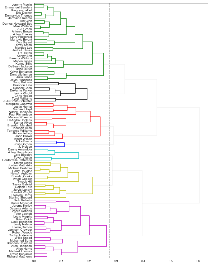
I churched up this dendrogram a little (for more, again, see this post for some ideas), but I mainly used it to eyeball-test where to “cut” and pick my number of clusters. I picked a cutline of 0.27 which seemed like a sweet spot to me, and gave 7 clusters.

ac = AgglomerativeClustering(n_clusters=7, linkage='ward').fit(zm)
np.bincount(ac.labels_)

array([ 5, 29, 14,  8, 22,  3, 14])

These clusters map to the dendrogram above — for example the cluster of 3 (group 6) is Mike Evans, Josh Gordon, and JJ Nelson — but let’s see if we can characterize these player groupings.

To visualize that, I’m going to plot the average distribution within each grouping (i.e. cluster) compared with the average league distribution. This may help me interpret the unique properties of a group better than just visualizing all the distributions at once. Here goes:

fig, axs = plt.subplots(len(np.unique(ac.labels_)), 1, 
                        sharex=True, figsize=(10,10))

cols = list('mycbrkg')  # same as dendrogram
avgd = z.iloc[:,1:-1].mean(axis=0)
for k,i in enumerate(np.unique(ac.labels_)):
    avgi = z[ac.labels_==i].iloc[:,1:-1].mean(axis=0)
    axs[k].bar(range(1,13), avgi - avgd, 0.8,
               color=cols[k], 
               label=i)
    axs[k].plot([0,13], [0,0], 'k-', lw=0.5)
    axs[k].text(11, 0.03, 'Group %d' % (i+1), fontsize=14)
    axs[k].set_ylim([-0.1, 0.1])

axs[-1].set_xlabel('Yardage', fontsize=14)
axs[-1].set_xticks(range(1,13))
axs[-1].set_xticklabels(z.columns[1:-1])
fig.text(0.04, 0.5, 'Difference from league avg', 
         va='center', rotation='vertical', fontsize=14)
  
axs[0].set_title('Clustering NFL Wide Receivers by Yardage Rates', fontsize=16)
plt.show()

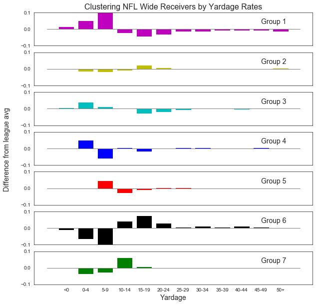
Very interesting. Let’s try to label these groups based on their distribution as compared to the league average. See if the player groupings feel right to you:

Group 1 are the checkdown kings. They excel at short yardage, at the expense of anything else. Players in this group include the one, the only, Cole Beasley, along with Cordarelle Patterson (has to be the play calling), Danny Amendola, Tavon Austin, and Adam Humphries.
Group 2 appears to be the star player group: consistent everywhere, above average in the explosive 15-25 yd range, and dangerous in the 50+ range. This group includes AJ Green, Julio Jones, Larry Fitzgerald, and Antonio Brown, and also some second-tier solid+dangerous players like TY Hilton and Demaryius Thomas.
Group 3 is like the slightly-more-dangerous version of Group 1. Most of their action comes from short plays, but they hit big plays at about a league average rate. Here’s Tyreek Hill, Stefon Diggs, Golden Tate, Nelson Agholor and some others.
Group 4 are the big-plays-only-please group. They are stand-outs in the 25+ plays, but the bulk of their plays are in the <5 yd range. Here we have Doug Baldwin, Randall Cobb, Chris Hogan, …
Group 5 is a first-down-and-then-some group. Almost perfectly average everywhere except in that 5-9 yd range, or 20-30 yd range. Here’s Allen Hurns, Mohamed Sanu, Odell Beckham, et al.
Group 6 is an exciting, select bunch, with the bulk of their plays at 10+ yds. Only three in this outlier group: JJ Nelson, Josh Gordon, and Mike Evans.
Group 7 is the slightly less exciting and less exclusive version of Group 6, with Brandon Marshall, DeAndre Hopkins, Keenan Allen, Paul Richardson, …

Parting thoughts

My ulterior motive for this post was to try to explain why “82% of Player X’s catches have been <15 yards” does not imply “Player X is not a deep threat.” In general, it seems like a good heuristic, and it’s certainly true for Cole Beasley, but it can be misleading: first of all, this fact doesn’t preclude the other 18% of Player X’s catches from being 50 yarders, and second, there are players where this is nearly true: for example, 76% of Tyreek Hill’s catches, 67% of Doug Baldwin’s catches, and 69% of Randall Cobb’s catches are less than 15 yards. I don’t think it’d be controversial to call those players dangerous.

Other thoughts: we could have instead looked at the distribution of yards per game, instead of yards in different amounts. Would we get similar clusters? I also didn’t even go into expected points added, even though we got that info for free during the scraping process. It might also be interesting to separate out yards and yards after catch: guys like Golden Tate or Odell Beckham might start to separate a bit.

Hopefully you’ve enjoyed this post. If you want to learn more about pandas, check out my post here, and if you want to scratch the fantasy football itch, check out this post or this post and the two follow-ons.

Feedback always welcome.