Steven Morse personal website and research notes
Anything you can do, I can do (kinda). Tidyverse pipes in Pandas
Written on August 8th, 2018 by Steven MorseI do most of my work in Python, because (1) it’s the most popular (non-web) programming language in the world, (2) sklearn is just so good, and (3) the Pythonic Style just makes sense to me (cue “you … complete me”). HOWEVAH, if R’s tidyverse + ggplot2 isn’t still the undisputed King of data wrangling and plotting, then I’m a monkey’s uncle.
And so I find myself constantly attempting to achieve tidyverse-style, idiomatic streamlining in my Jupyter notebook or Colab sessions. This blog post is my attempt to share a couple lessons learned with the world — at least, the parts of the world who work in pandas and have perhaps an exposure to the #tidyverse #rstats.
This blog is not an all-encompassing intro to pandas — a more thorough intro is here, a great Rosetta Stone of pandas/dplyr is here, and there’s an entertaining tour of Python viz options here.
My mission is to see how much I can make pandas+seaborn feel like tidyverse+ggplot2. In particular, one of the great joys of working in the tidyverse is being able to do a complicated wrangling job in one continuous pipe, without any intermediary objects. So my main goal in this post is to see how much single-chain tidyverse wrangling I can do as single-chain pandas. Tom Augspurger does an intro here, but I’d like to push the envelope a little and explore the differences from an R user’s perspective: there’s a lot of one-to-one mappings from tidyverse-to-pandas, I’d like to see where exactly it breaks down.
tl;dr tidyverse + ggplot2 is better, but we can get 90% of the way there in Python with just pandas + seaborn (thus the title of this blog…), without needing any bleeding-edge copy-cat packages like plotnine, dplython, ggpy, etc.
The basics
I’ll use the diamonds dataset since it’s available through ggplot2 (here’s a description of the fields) and seaborn, so there’s lots of examples on both sides of the house. You can also grab it here.
%matplotlib inline
import matplotlib.pyplot as plt
import seaborn as sns
import numpy as np
import pandas as pd
sns.set_style('white')

df = sns.load_dataset('diamonds')
df.head()
	carat	cut	color	clarity	depth	table	price	x	y	z
1	0.23	Ideal	E	SI2	61.5	55.0	326	3.95	3.98	2.43
2	0.21	Premium	E	SI1	59.8	61.0	326	3.89	3.84	2.31
3	0.23	Good	E	VS1	56.9	65.0	327	4.05	4.07	2.31
4	0.29	Premium	I	VS2	62.4	58.0	334	4.20	4.23	2.63
5	0.31	Good	J	SI2	63.3	58.0	335	4.34	4.35	2.75
And here’s a cool site on the 4 C’s of diamond quality because I know y’all are too lazy to google it!
Let’s start with pandas vs. dplyr …
The basic mapping of dplyr to pandas is:
dplyr |
pandas |
|---|---|
mutate |
assign |
select |
filter |
rename |
rename |
filter |
query |
arrange |
sort_values |
group_by |
groupby |
summarize |
agg |
There are of course many others (on both sides of the table), but this is a good start.
Next up: the beloved “pipe” operator %>% in the Tidyverse (actually due to the magrittr package) allows you to turn nested operations into chains, like this:
# turn this ...
filter(select(df, carat, color), color == 'E')

# into this ...
df %>%
  select(carat, color) %>%
  filter(color == 'E')
which is lovely to read. We can achieve the same effect in pandas because data is represented as a class instance of pandas.DataFrame, so we can do successive method calls like this:
(df
 .filter(['carat', 'color'])
 .query('color == "E"')
 .head(3))
	carat	color
1	0.23	E
2	0.21	E
3	0.23	E
Of note: gotta wrap the whole thing in parantheses (what is this, Lisp?), or else end each line with a backslash (ugh). The quotes in query need to be single-outside, double-inside (or the reverse), not all the same. You need to pass a list of columns to filter-in (dplyr: select). Everything’s in quotes, all the time, no tidyeval quosures or whatnot here.
Overall though, our mapping is right on track so far.
Let’s try a slightly trickier one.
# dplyr
df %>%
  select(starts_with('c')) %>%
  filter(cut %in% c('Ideal', 'Premium')) %>%
  group_by(cut, color, clarity) %>%
  summarize(avgcarat = mean(carat, na.rm=TRUE),
            n = n()) %>%
  arrange(desc(avgcarat)) %>%
  head()
… or …
# python
(df
 .filter(regex='^c')
 .query('cut in ["Ideal", "Premium"]')
 .groupby(['cut', 'color', 'clarity'])
 .agg(['mean', 'size'])
 .sort_values(by=('carat', 'mean'), ascending=False)
 .head())
                            carat
                        mean      size
cut      color	clarity
Ideal    J		  I1		  1.990000	2
Premium	 I		  I1		  1.605833	24
	J		I1		  1.578462	13
			SI2		  1.554534	161
Ideal	   H		  I1		  1.475526	38
Not bad, and we are almost exactly one-to-one with dplyr, but some things to note:
- We had to resort to regular expressions. We could have replaced the 2nd line with
.filter(df.columns[df.columns.str.startswith('c')]), but that is definitely worse. Or led off with the slice(df[df.columns.str.startswith('c')]...)but that’s clunky and ruins the chain pattern. Just learn a little regex I guess? - The
querycommand is really nice and idiomatic (dare I say better???). - Two things happening behind the scenes of that
aggcommand. First, it silently drops non-numeric columns since we asked for a mean, which means just the carat column is left, which is all we wanted anyway. But if, for example, color were numeric, it’d be giving us the means for that column too. The “size” command is analogous ton(), and measures the number of rows in a group for a particular column, in this case for carat. This is a bit weird to me, “size” should not be a sub-property of carat, it should be its own column, but there doesn’t appear to be a way to do that (unless you create a dummy column with.assign(n=1) ... .agg({'n': 'size'})). - We now have a
pandas.MultiIndexhappening in the rows and columns. We can get rid of the row multi-index by callingreset_index()(helpful later for plotting), similar toungroup()in dplyr, but I’m not sure how to “flatten” the columns in a chain like this. This is what leads to the tuple('carat', 'mean')insort_values.
I think this little maneuver captures the essence of the differences between dplyr and pandas. Basically, pandas can do it, but it’s not “opinionated” about how you do things (Hadley’s words, not mine) and therefore the way(s) to do it are not as streamlined.
… and a little tidying
I think where ggplot2 really started to sing for me was when I (finally) figured out how “tidy” data worked, and how to employ tidyr::gather and tidyr::spread in a data wrangle chain.
For example, say we want to plot separate histograms of the x, y, and z columns. Well, we could loop through 3 ggplot commands, specifying a different color each time (this is the base R or matplotlib approach, and honestly I don’t mind it), or we can gather the x-y-z columns into long format so that each diamond corresponds to 3 rows: one for x, one for y, one for z. Now we have a column designating whether it’s x, y, or z, and a column with the corresponding value. Behold:
# tidyr
df %>%
  select(x, y, z) %>%
  gather(key=dim, value=mm) %>%
  head()
# A tibble: 6 x 2
  dim      mm
  <chr> <dbl>
1 x      3.95
2 x      3.89
3 x      4.05
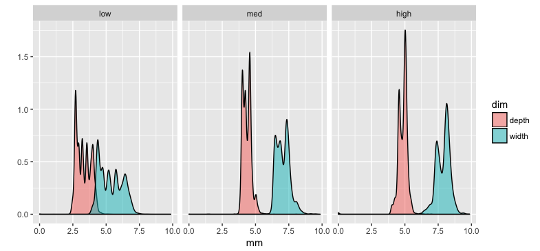
which sets us up to do a “grammar of graphics”-style plot like this
df %>%
  mutate(price.cat = cut(price, breaks=3, labels=c('low', 'med', 'high'))) %>%
  select(price.cat, width=x, depth=z) %>%
  gather(key=dim, value=mm, -price.cat) %>%
  filter(mm < 10) %>%
  ggplot(aes(x=mm, fill=dim)) +
  geom_density(alpha=0.5) +
  facet_wrap(~price.cat) +
  ylab('')
For pandas the equivalent is
tidyr |
pandas |
|---|---|
gather |
melt |
spread |
pivot |
Also in the pandas toolbox is stack and unstack, and pivot_table, depending on the structure of the DataFrame. See this post or the docs for a little more thorough discussion.
Can we reproduce the 9-line beauty from above in pandas? Let’s start with the data structure:
(df
 .assign(pricecat = pd.cut(df['price'], bins=3, labels=['low', 'med', 'high']))
 .filter(['x', 'z', 'pricecat'])
 .rename(columns={'x': 'width', 'z': 'depth'})
 .melt(id_vars=['pricecat'], value_vars=['width', 'depth'],
       var_name='dim', value_name='mm')
 .head())
	pricecat	dim		mm
0	low			width	3.95
1	low			width	3.89
2	low			width	4.05
3	low			width	4.20
4	low			width	4.34
We did it! It’s almost identical! We did have to add a line to rename columns, since dplyr’s select was cheating by doing double-duty as rename. But biggest difference, to me, is that melt wants you to specify the list of where information is coming from, whereas tidyr::gather wants you to specify where the information is going to. This is fine by me though, and maybe even makes more sense.
Now to plot it.
Visualization
First, a straightforward approach. Second, a trick.
Vanilla
A straightforward thing to do would be to just save the DataFrame and then plot it, for example,
df2 = (df
 .assign(pricecat = pd.cut(df['price'], bins=3, labels=['low', 'med', 'high']))
 .filter(['x', 'z', 'pricecat'])
 .rename(columns={'x': 'width', 'z': 'depth'})
 .melt(id_vars=['pricecat'], value_vars=['width', 'depth'],
       var_name='dim', value_name='mm')
 .query('2 < mm < 10'))

g = sns.FacetGrid(data=df2, col='pricecat', hue='dim')
g.map(sns.kdeplot, 'mm', shade=True, alpha=0.5).add_legend()
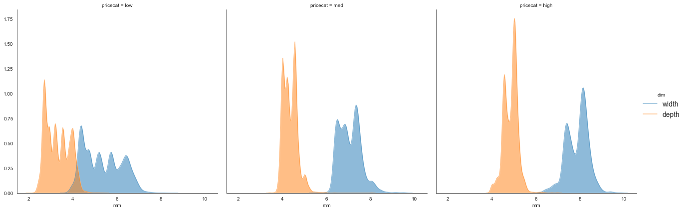
The pipe + seaborn trick
But we can do better. pandas.DataFrame exposes a pipe method that allows us to pipe in any method we want. To include: plotting methods.
(df
 .assign(pricecat = pd.cut(df['price'], bins=3, labels=['low', 'med', 'high']))
 .filter(['x', 'z', 'pricecat'])
 .rename(columns={'x': 'width', 'z': 'depth'})
 .melt(id_vars=['pricecat'], value_vars=['width', 'depth'],
       var_name='dim', value_name='mm')
 .query('2 < mm < 10')
 .pipe((sns.FacetGrid, 'data'),
       col='pricecat', hue='dim', height=6)
 .map(sns.kdeplot, 'mm', shade=True, alpha=0.5)
 .add_legend(fontsize=14))
I’ll omit the image because it’s essentially identical to the previous. The main trick is the tuple (sns.FacetGrid, 'data') that sends the DataFrame to the data arg of FacetGrid.
But how cool is that: this is nearly identical to a tidyverse+ggplot approach, almost line-by-line. Biggest difference is perhaps having to facet first. I am really satisfied that I can wrangle a DataFrame and pipe it directly into a viz.
Here’s another for good measure, with some longer query and FacetGrid commands.
(df
 .query('cut in ["Ideal", "Good"] & \
         clarity in ["IF", "SI2"] & \
         carat < 3')
 .pipe((sns.FacetGrid, 'data'),
       row='cut', col='clarity', hue='color',
       hue_order=list('DEFGHIJ'),
       height=6,
       legend_out=True)
 .map(sns.scatterplot, 'carat', 'price', alpha=0.8)
 .add_legend())
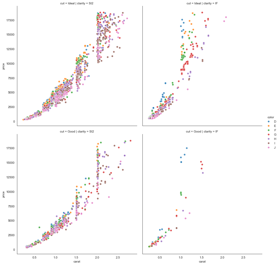
We have the not-surprising result that price increases super-linearly with caret. Maybe interesting is how steeply the increase occurs with “internally flawless” (IF) diamonds, regardless of cut-quality, compared with “slightly included” diamonds.
Taking things too far
I’ve said it before and I’ll say it again: sometimes this type of method-chaining feels like trying to line up all the targets perfectly so you can get everything you want with one shot. And yet often it’s easier, nicer, even faster, to just walk over and smash the targets one by one with a hammer. And by hammer I mean matplotlib and a for-loop.
Here’s an example. Let’s say we want to visualize a scatterplot of price vs. carat for all diamonds in the dataset, but highlight the datapoints corresponding to the highest quality combination of cut/clarity. Here’s the most elegant way I can figure to do this as a “one-liner”:
fig, ax = plt.subplots(1,1, figsize=(8,8))
pal = dict(zip(df['color'].unique(), sns.color_palette('Set1', desat=.9)))
pal['Other'] = (1,1,1)

(df
 .assign(nice = np.where((df['cut']=='Ideal') & (df['clarity']=='IF'), df['color'], 'Other'))
 .sort_values(by='nice', ascending=False)
 .pipe((sns.scatterplot, 'data'),
       x='carat', y='price',
       hue='nice', hue_order=np.append('Other', list('DEFGHIJ')),
       palette=pal,
       alpha=0.8,
       edgecolor=(0.92,0.92,0.92),
       ax=ax))
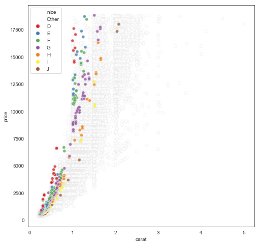
Note the contortions we have to undergo to make this work: a new column with color for the special group and “Other” for others (seems sensible), sort so the “Other” rows are first and thus get plotted first in the scatterplot (hmm a little sketchy but ok nice trick), create a custom palette with white for “Other”, then put a very light edge around all points so we can see the white ones but they’re not distracting.
Exhausting, and in this case, a little silly. Here’s a hammer-smash-bottle approach that creates nearly an identical plot (perhaps an even better one):
df2 = (df
 .assign(nice = np.where((df['cut']=='Ideal') & (df['clarity']=='IF'), df['color'], 'Other')))

fig, ax = plt.subplots(1,1, figsize=(8,8))

ax.scatter(data=df2.query('nice == "Other"'), x='carat', y='price',
           c=[[0.92,0.92,0.92]], s=20, alpha=0.2)

sns.scatterplot(data=df2.query('nice != "Other"'), x='carat', y='price',
                hue='color', hue_order=list('DEFGHIJ'),
                palette='Set1', s=30, alpha=0.9, ax=ax)

So it involved creating a duplicate of df, which might be prohibitive for very large or streaming datasets, but it’s way easier to understand, write, debug, etc.
Parting thoughts
- Nothing requires us to use seaborn, we could have used
matplotlibin thosepipecommands. (Andpyplot.scattersupport column name indexing now!) Also, pretty sure you could also useAltairor other plotting methods as well but I haven’t yet tried. - Inexperienced musing:
tidyverseallows a mix of quoted and unquoted references to variable names. In my (in)experience, the convenience this brings is accompanied by equal consternation. It seems to me a lot of the problems solved bytidyevalwould not exist if all variables were quoted all the time, as in pandas, but there are likely deeper truths I’m missing here…
Thanks for reading! Feedback always welcome.
Written on August 8th, 2018 by Steven Morse