Bayesian Coin Flipping

Written on December 30th, 2023 by Steven Morse

This post will walk through a Bayesian treatment of coin flipping. Yes, yes, this has been done a billion times on the internet and in every probability textbook ever written, but I’m doing it again here because 1) this is for future me as a reference, and, 2) I think I’m better than all those other resources at explaining it (okay fine I’m not) – but specifically, I’ll be as explicit as possible with both math and code throughout, show derivations, etc.

The Premise

Let’s say we have a sequence of $n$ coin flips, and trying to determine what will happen next.

One natural way is to count the number of heads so far, divide it by the total, and use this as our probability estimate $\hat{\theta}$ of the next flip being a head. So if we saw 16 heads in 20 flips, we’d say the probability of seeing the next one turn up heads is $\hat{\theta} = 16/20 = 0.8$. (In fact, this is the maximum likelihood estimate (MLE) of the probability of seeing a head, which we can compute in a little more principled way, which I’ll save for later.)

One problem with this arises with smaller numbers – after two flips, both heads, are we really saying we’re 100% sure the next will be a head too? Obviously not. Another is we have no clear way of incorporating any prior knowledge of unfairness into the estimate.

Overall, this is the frequentist approach. There are ways to adjust for small numbers, and bias, but to me they seem a little ad hoc. Another way is to use a Bayesian approach.

In the Bayesian approach, we treat the probability of heads, $\theta$, as a random variable itself! This may seem very natural, but it seems to really rankle the mental model of folks used to working in frequentist paradigms. The variable, random or not, is modeling the internal heft and balance of the coin, its propensity to land on one side or the other – although these are fixed, physical qualities, it seems natural to treat their manifestation as a chance of some outcome, as something with uncertainty, as a random variable.

Anyway, we can compute the distribution of $\theta$, taking into account the data $D$ (the history of coin flips), using Bayes’ theorem:

\[P(\theta \ \vert \ D) = \frac{P(D\vert \theta) \ P(\theta)}{P(D)}\]

This says, the posterior of $\theta$, conditioned on the data, is equal to the likelihood of the data occurring given our distribution over $\theta$, times our prior on $\theta$, normalized by the marginal likelihood of the data.

Defining distributions

We need to define the terms in this formula. Specifically, we need to assign distributions to the different random variables.

Likelihood of the evidence (given the prior)

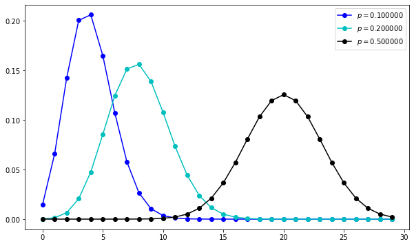
Starting with the data. Given a sequence of $n$ coin flips, define the random variable $X$ to represent the number of “heads”. Let the probability of a head be $\theta$. Then, the probability of $X$ being a particular $k$ given $\theta$ (i.e. the likelihood) is a binomial distribution.

\[\begin{align*} X\vert \theta &\sim \text{Binom}(n, \theta) \\ P(X=k \ \vert \ \theta) &= \begin{pmatrix}n \\ k\end{pmatrix} \theta^k (1-\theta)^{n-k} \end{align*}\]

The binomial distribution is a very intuitive extension of a set of Bernoulli RVs. A Bernoulli RV can be either 1 or 0 (say, heads or tails), for example $P(\tilde{x}=1) = \theta$. So if you have $n$ of these RVs, the probability that $k$ of them turn up heads is $\theta^k$ times the probability $n-k$ turn up tails, $(1-\theta)^{n-k}$, and this can happen “n choose k” ways (for example, with 3 flips, 1 head, we count HTT, THT, TTH = 3 ways). (This binomial coefficient is the namesake of the distribution.)

Let’s take a look at some distributions of $X$ over $k$ for different values of $\theta$.

import matplotlib.pyplot as plt
import numpy as np
import scipy.stats

fig, ax = plt.subplots(1,1, figsize=(10,6))

xs = np.arange(0, 30)
n = 40
for p, c in zip([0.1, 0.2, 0.5], ['b', 'c', 'k']):
    rv = scipy.stats.binom(n, p)

    ax.plot(xs, rv.pmf(xs), marker='o', color=c, linestyle=None, label=r'$p=%f$' % p)
    # ax.vlines(xs, 0, rv.pmf(xs), colors=c, lw=1)

ax.legend()
plt.show()

Prior

Next, we need to pick a distribution to represent our prior over $\theta$, the term $P(\theta)$. Let’s use a beta distribution,

\[\begin{align*} \theta &\sim \text{Beta}(\alpha, \beta) \\ P(\theta) &= \frac{1}{B(\alpha,\beta)}\theta^{\alpha-1}(1-\theta)^{\beta-1} \end{align*}\]

where $B(\alpha, \beta)$ is the Beta function, closely related to the Gamma function.

What does the beta distribution look like for different values of $\alpha$ and $\beta$, you ask?

fig, ax = plt.subplots(1,1, figsize=(10,6))

xs = np.linspace(0, 1, 100)
for (a,b), c in zip([(1,1), (2,2), (3,1), (2,3)], ['b', 'c', 'g', 'k']):
    rv = scipy.stats.beta(a, b)

    ax.plot(xs, rv.pdf(xs), marker=None, color=c, linestyle='-', 
            label=r'$\alpha=%d, \ \beta=%d$' % (a,b))

ax.legend()
plt.show()

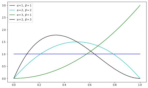
The hyperparameters $\alpha$ and $\beta$ act as pseudo-counts of the heads/tails flipping. Notice when they’re both 1, we get a uniform distribution. As they stay equal, but increase, we become increasingly peaked around the mode of $\theta=0.5$ (like a fair coin). When $\alpha$ is higher, we get a lot of probability mass on upper values for $\theta$, indicating a proclivity for heads.

Marginal likelihood

Lastly, we need to calculate that denominator, which has a tendency to get nasty in Bayesian treatments. Fortunately, since we’ve chosen a prior distribution conjugate to our likelihood, we can do

\[\begin{align*} P(X) &= \int_0^1 P(X\vert \theta)P(\theta) \ d\theta \\ &= \begin{pmatrix}n \\ k\end{pmatrix} \frac{1}{B(\alpha,\beta)} \ \int_0^1 \theta^{k+\alpha-1}(1-\theta)^{n-k+\beta-1} \ d\theta \end{align*}\]

We notice that the integrand looks like a beta distribution with $\alpha' = k+\alpha$ and $\beta' = n-k+\beta$, so we can do the little maneuver (being very explicit here) of multiplying by a “1” consisting of the appropriate Beta functions for this new beta distribution, and using the fact that PDFs integrate to 1 over their support:

\[\begin{align*} P(X) &= \begin{pmatrix}n \\ k\end{pmatrix} \frac{B(k+\alpha, n-k+\beta)}{B(\alpha,\beta)} \ \int_0^1 \frac{1}{B(k+\alpha, n-k+\beta)} \theta^{k+\alpha-1}(1-\theta)^{n-k+\beta-1} \ d\theta \\ &= \begin{pmatrix}n \\ k\end{pmatrix} \frac{B(k+\alpha, n-k+\beta)}{B(\alpha,\beta)} \end{align*}\]

Putting it all together

Combining the prior, likelihood, and marginal together, we can analytically derive an expression for the posterior (not showing all steps here because it is very straightforward):

\[P(\theta \vert X) = \frac{1}{B(k+\alpha, n-k+\beta)} \theta^{k+\alpha-1}(1-\theta)^{n-k+\beta-1}\]

which we recognize as a beta distribution,

\[\theta \vert X \sim \text{Beta}(k+\alpha, n-k+\beta)\]

We’ve already seen what a beta distribution looks like. Let’s experiment with what happens for different priors and observations.

Playing with posteriors

Let’s first assume a prior of $\alpha=2$, and $\beta=2$. Then let’s flip the coin $n=5$ times, and say we observe $k=2$ heads. This gives:

fig, ax = plt.subplots(1,1, figsize=(10,6))

a, b = 2, 2
n, k = 5, 2

prior     = scipy.stats.beta(a, b)
posterior = scipy.stats.beta(k + a, n - k + b)

xs = np.linspace(0, 1, 100)
ax.plot(xs, prior.pdf(xs), marker=None, color='c', linestyle='-', label='Prior')
ax.plot(xs, posterior.pdf(xs), marker=None, color='k', linestyle='-', label='Posterior')

ax.set(xlabel='Probability of heads')

ax.legend()
plt.show()

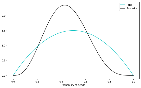
We’ve started with an assumption of a fair coin, loosely speaking, and just saw it flip heads 2 out of 5 times, so we have an updated view that the coin may be skewed toward heads, around 0.4 or so, but not very strongly so.

Let’s watch this posterior converge as we flip more and more times:

fig, ax = plt.subplots(5,1, figsize=(12,6), sharex=True)

a, b = 2, 2
n, k = 40, 25
xs = np.linspace(0, 1, 100)

prior     = scipy.stats.beta(a, b)
ax[0].plot(xs, prior.pdf(xs), marker=None, color='c', linestyle='-')

for i, (n,k) in enumerate([(5,2), (10, 5), (20, 11), (40, 25)]):
    posterior = scipy.stats.beta(k + a, n - k + b)
    ax[i+1].plot(xs, posterior.pdf(xs), marker=None, color='k', linestyle='-', label='Posterior')

plt.show()

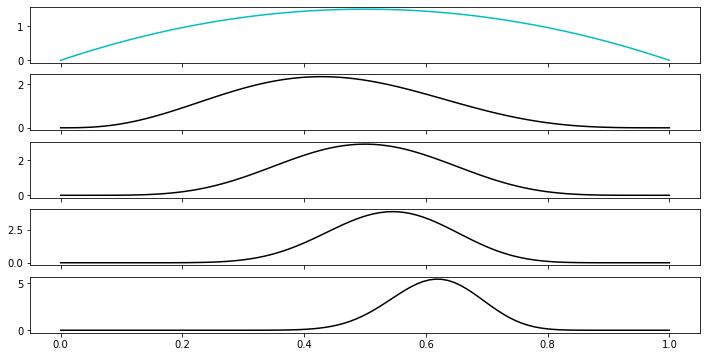
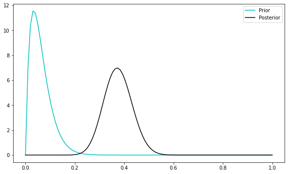
So you can see we are starting to be confidently peaked the other direction around a slightly “loaded” coin, with $\theta$ around $25/40 = 0.62$. But if we’d started with a different prior, thinking for example the coin was biased the other direction, we’d have skewed this conclusion and be less certain:

fig, ax = plt.subplots(1,1, figsize=(10,6))

a, b = 2, 30
n, k = 40, 25

prior     = scipy.stats.beta(a, b)
posterior = scipy.stats.beta(k + a, n - k + b)

xs = np.linspace(0, 1, 100)
ax.plot(xs, prior.pdf(xs), marker=None, color='c', linestyle='-', label='Prior')
ax.plot(xs, posterior.pdf(xs), marker=None, color='k', linestyle='-', label='Posterior')

plt.legend()
plt.show()

Predicting

So far we’ve just introspected on how to assess the value of $\theta$. What we’d really like to do is be able to say something about the next coin flip $\tilde{x}$, given all the data $X$. We could first consider what $\tilde{x}$ is likely to be given our knowledge of $\theta$, that is, $P(\tilde{x}\vert \theta)$. This flip is a Bernoulli RV, so very simply $P(\tilde{x}=1\vert \theta) = \theta$.

MAPs

It may be tempting to use a point estimate of $\theta$ here. For example, we could use the maximum of the posterior distribution. This is called the maximum aposterior estimate, or MAP estimate.

Since our posterior is a beta distribution, the maximum is the mode. Compute the derivative of the distribution, set it to zero, and solve for $\theta$ … it’s honestly a bit tedious of a calculation, I recommend just checking it out somewhere, but the punchline is:

\[\hat{\theta}_{\text{MAP}} = \frac{k + \alpha - 1}{n + \alpha + \beta - 2}\]

This is very intuitive. We’re taking the frequentist estimate of $k/n$ and augmenting it a little by our prior pseudocounts. The decrements of -1 and -2 ensure that a uniform prior of $\alpha=\beta=1$ returns exactly the estimate $k/n$.

This is an example of a classic Bayesian point to frequentists: your estimate is just a special case of a point estimate of our method!

Predictive posteriors

Still, this MAP business should be a little unsatisfying. We’re discarding all the information we worked so hard for, by dropping down to a point estimate. Wouldn’t we prefer to incorporate all the data, and prior on $\theta$, into our estimate of $\tilde{x}$?

Yes – specifically, we’d like an expression for $P(\tilde{x}\vert X)$.

This is called the posterior predictive distribution. We can, in theory, compute it with:

\[p(\tilde{x}\vert X) = \int_{\theta} p(\tilde{x}\vert \theta) \ p(\theta\vert X) \ d\theta\]

This is called marginalizing over $\theta$ and – speaking loosely – captures everything we know about $\theta$ and $X$ into a distribution over $\tilde{x}$, by sort of averaging over $\theta$.

In practice, we often have a potentially nasty integral to calculate. But in this case, we actually get a version of the MAP, which I won’t reproduce here, check out these lecture notes for a little more detail.

The posterior predictive is not actually very exciting in this setting, but I encourage you to check it out in a linear regression setting for a richer view.

That’s all for today! Thanks for reading.