Poisson process simulations in Python - Part 1

“I am my own experiment. I am my own work of art.” — Madonna

I love to tinker and experiment while I’m learning a concept – it helps me build intuition and confidence in the mathematics, and helps bring abstract proofs down to earth. In this post, I’ll explore the Poisson process by going a little light on the math and heavier on simulation and building intuition.

I’ll be working in Python, and use primarily the matplotlib and numpy libraries:

import matplotlib.pyplot as plt
import numpy as np

My goal for this post’s tone and pace is to target someone with an intermediate, but not advanced, understanding of both probability and Python. We’ll cover some background and build intuition with the base process. In the next post, we’ll loosen and modify several of the core assumptions and explore more flexible versions of this process.

We may define a Poisson process in two ways: via the Poisson distribution, or via the exponential. It turns out they’re equivalent definitions, each yielding interesting properties, and each enabling different approaches to simulation as we’ll see later. EDIT: I originally structured this as “via the Poisson distribution” first, then “via the exponential”, but decided to swap this order, felt like it read better.

Via the exponential distribution

The Poisson process is a sequence of points — called events or arrivals — along the positive real line such that the number of arrivals \(N\) occurring in any interval \((a,b]\) follows a Poisson distribution with shape parameter \(\Lambda\). But let’s come back to the Poisson distribution later.

Another way to define a Poisson process, is a sequence of arrivals such that each interarrival time is an exponential random variable with parameter \(\lambda\). That is, with \(\Delta_k t = t_{k+1} - t_k\),

That probability form \(e^{-x}\) indicates we expect mostly short interarrival times, occasionally some longer stretches, and almost never anything extreme. On average, you expect to wait about \(1/\lambda\).

For example, say you are observing cars passing by on a rural road, and the cars pass at a rate of \(\lambda = 10\) cars per day. It might be natural to model the wait between cars as following an exponential distribution – in this case, with an average (mean) wait of \(1/10\)-th of a day.

Let’s try a quick simulation of this and make sure nothing seems fishy (ha!).

rate, T = 10, 1

# grab a bunch of interarrival times
dt = np.random.exponential(1/rate, 100)  

# compute successive sums to create a sequence of arrival times
ts = np.cumsum(dt)  

# remove events that exceed the horizon
ts = ts[ts < T]  

(Equivalently, we could just as well have iteratively built the list ts of arrival times, appending samples from the exponential, but using cumsum is more efficient. Either way, we get a sequence something like this:)

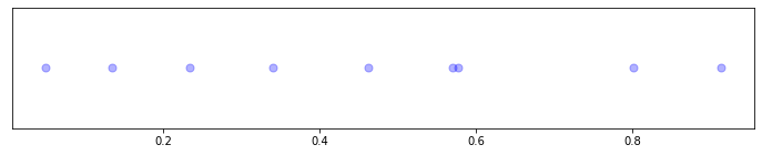
Nice. Each blue dot is the passing of a car on our rural road, over the course of one day.

Sidequest: Exploring memorylessness

The following sidequest is not immediately relevant to the main thrust of understanding of the Poisson process, but is, nevertheless, very weird and interesting.

One can show that, because the interarrival times have this distribution, not only is each interarrival time independent of each other, but something more: the interarrival times are memoryless. That is to say, given that you know time \(y\) has passed, the residual remaining time left of \(X\) has the same distribution that it would if you didn’t know \(y\) had passed! In math,

And since \(\text{Pr}(X-y>x) = \text{Pr}(X>x+y)\), we can prove this simply with

This property is a bit strange. A typical illustration is to imagine waiting at a bus stop, where your expectation of the wait is, say, 2 hours, and you’re using the exponential distribution as your model of waiting time. Now 5 hours elapses. Your expectation of the remaining wait to a bus, despite knowing that 5 hours has already elapsed, is still 2 hours. The random variable controlling the remaining time has no memory of the past wait!

Via the Poisson distribution

Ok, let’s explore another view on the Poisson process.

As we said, the Poisson process is a sequence of events such that the number of arrivals \(N\) occurring in any interval \((a,b]\) follows a Poisson distribution with shape parameter \(\Lambda\). Explicitly,

And we define \(\Lambda = \lambda T\) with \(T=b-a\), and \(\lambda\) the rate (we can show this is the same parameter as before, with the exponential). For now, let’s think of \(T\) as simply a length (but we can expand to a broader sense of measure: area, volume), and \(\lambda\) as a constant (but we can expand, for example to vary with time).

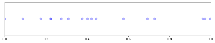
Let’s put this into action. Let’s grab a sample from the Poisson distribution with shape \(\Lambda = \lambda T\), and place those points uniformly at random along an interval of length \(T\).

rate, T = 10, 1

NT = np.random.poisson(rate * T)
ts = np.random.uniform(0, T, size=NT)
ts = np.sort(ts)  

# note: we don't have to sort for the visualization,
# but we need to for the dataset to make sense as a sequence

fig, ax = plt.subplots(1,1, figsize=(12,2))
ax.scatter(ts, [0]*len(ts), c='b', s=50, alpha=0.3)
ax.set(xlim=[0,T])
ax.get_yaxis().set_visible(False)

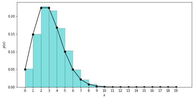
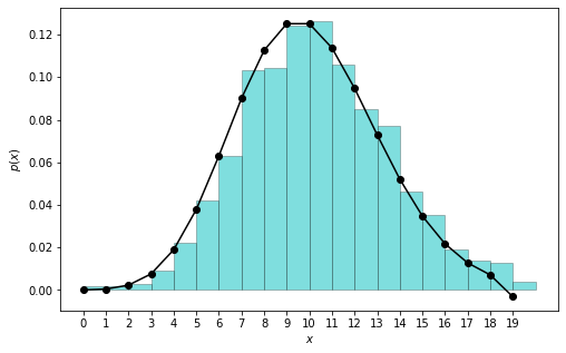
For fun, let’s explore the Poisson distribution a bit. Here’s the discrete Poisson distribution, with shape \(\Lambda = 3\), computed both directly from the PMF and as a histogram of samples:

# both `math` and `numpy` have `factorial`s,
# but this one allows vectorized computation
from scipy.special import factorial

shape = 3

# compute the PMF directly
# note: `scipy` has PMF/PDFs for all common dists, but
# it's more illustrative to code ourselves
def poisson_pmf(x, shape):
    return (np.power(shape, x) / factorial(x)) * np.exp(-shape)
xs = np.arange(0, 20)
ps = poisson_pmf(xs, shape)

# get samples from the distribution
samples = np.random.poisson(lam=shape, size=10000)

fig, ax = plt.subplots(1,1, figsize=(10,5))
ax.plot(xs, ps, 'ko-')
ax.hist(samples, bins=20, range=(0,20), density=True, 
        color='c', alpha=0.5, edgecolor='k', linewidth=0.5)
ax.set(xlabel=r'$x$', ylabel=r'$p(x)$')
ax.set_xticks(range(0,20))

And we might as well check a few other shapes:

fig, ax = plt.subplots(1,1, figsize=(8,5))
shapes = [1, 5, 10]
colors = ['k', 'c', 'b']
labels = [r'$\Lambda=%d$' % s for s in shapes]
for s, c, lab in zip(shapes, colors, labels):
    ps = poisson_pmf(xs, s)
    ax.plot(xs, ps, marker='o', color=c, label=lab)
ax.legend(fontsize=14)
ax.set(xlabel=r'$x$', ylabel=r'$p(x)$')

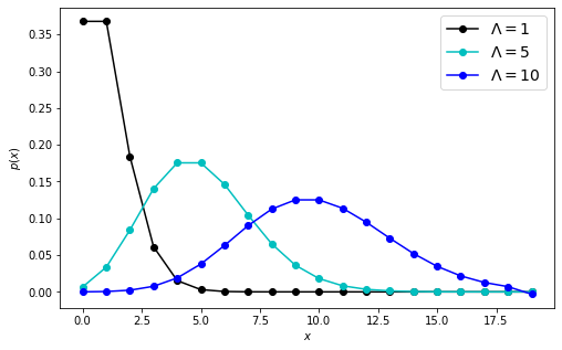
So we see it’s a well-behaved, thin-tailed, tractable little distribution with mean \(\Lambda\) and mode \(\lfloor \Lambda \rfloor\).

Returning to our example, if you recorded the number of cars passing by from before (with rate \(\lambda = 10\)), every day, for several months, and plot the distribution of these end-of-day totals, the distribution would match the Poisson distribution above with \(\Lambda = 10\).

By the way, the expected number of arrivals over any time \(T\) is, as you might expect, \(\Lambda = \lambda T\). This property also extends to higher dimensional versions of the process. The derivation is fun:

This result should feel very common sense. Using our example of cars passing on a rural road, with rate \(\lambda = 10\) cars per day, and you observe for \(T=2\) days, then you expect to see \(10\times 2 = 20\) cars.

The fact that the number of arrivals is Poisson distributed follows from the interarrival time definition, which we can show precisely with a short, but careful proof.

ORRRR, instead, let’s just experimentally verify that the two definitions consistently match, by generating a bunch of sequences using interarrival times, and checking the total events match the Poisson distribution.

rate, T = 10, 1
counts = []
for _ in range(1000):
    # -- this is our code from before -- #
    dt = np.random.exponential(1/rate, 100)  # grab a bunch of samples
    ts = np.cumsum(dt)
    ts = ts[ts < T]  # remove events that exceed the horizon 

    # all we care about now is total # of events
    counts.append(len(ts))  

# recompute our Poisson PMF
xs = np.arange(0, 20)
ps = poisson_pmf(xs, rate * T)

I’ll allow myself to be convinced.

Interlude

Recall we defined a Poisson process such that the count of arrivals over any interval is distributed Poisson. This is key. For our car example, in order to be a Poisson process, just as the end-of-day totals must match a Poisson distribution, the end-of-week totals must match a Poisson distribution (with \(\Lambda = 70\)) – and the end-of-hour, end-of-minute, etc.

Suppose not: imagine your day-totals are Poisson distributed, but they’re all packed into the first minute of the day! So the day-interval exhibits Poisson-iness on aggregate, but no interval does – this is obviously not Poisson.

Perhaps surprisingly, we ensured this didn’t happen when we placed the points uniformly at random along the interval. This seeming benign choice of placement was actually critical: it ensured the points would have a common distribution of interarrival times.

Let’s check this, that generating sequences by sampling \(N\) from the Poisson, and arranging uniformly at random, gives exponential interarrival times. This time we’ll compare the true and experimental CDFs (instead of PDFs), to avoid any fussing with binning.

rate, T = 10, 1

dts = np.array([])
for _ in range(1000):
    # -- this is our code from before --
    NT = np.random.poisson(rate * T)
    ts = np.random.uniform(0, T, size=NT)
    ts = np.sort(ts)

    # append all these interarrival times
    dts = np.append(dts, ts[1:] - ts[:-1])

# compute the (experimental) CDF of the data
ecdf_x = np.sort(dts)
ecdf_y = np.arange(len(ecdf_x)) / float(len(ecdf_x))

# compute the (exact) CDF of the exponential
xs = np.linspace(0, 1, 100)
exps = 1 - np.exp(-rate * xs)

fig, ax = plt.subplots(1,1, figsize=(8,5))
ax.plot(xs, exps, 'k-', label='CDF')
ax.plot(ecdf_x, ecdf_y, 'c-', label='ECDF')
ax.set(xlabel=r'$x$ (interarrival time)', ylabel=r'$F(x)$')
ax.legend(fontsize=14)

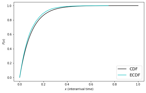
Checks out … but it’s obscuring a fact. We’d get the same concurrence between the ECDF of the interarrivals and the CDF of the exponential, even if we used a constant number of arrivals. Try switching out

# NT = np.random.poisson(rate * T)
NT = 10

You’ll get the same plot. The fact is that a uniform distribution of any number of points will yield exponentially distributed interevent times.

This may start to feel a bit circular, so let’s review what we know.

Review

Let’s recap.

Definition 1. A Poisson process is a sequence of arrivals such that interarrival times \(\Delta t_i\) are i.i.d with distribution \(\text{Pr}(\Delta t_i \leq x) = 1-e^{-\lambda x}\).

It just so happens, from this definition, we can show that the number of arrivals \(N(t)\) in any interval of length \(t\) is a Poisson random variable. We showed this experimentally, earlier. We’ll omit the actual proof though, since it’s no one-liner, and we set out to be “light on math” (sad!).

So, for our other definition:

Definition 2. A Poisson process is a sequence of arrivals such that the number of arrivals \(N(t)\) in any interval \(t\) is a Poisson random variable, \(\text{Pr}(N=k) = (\Lambda^k/k!) \ e^{-\Lambda}\), with \(\Lambda = \lambda t\).

Definition 2 is self-contained. However, unlike Definition 1, it doesn’t proscribe how the arrivals could be simulated. It turns out, that distributing any number of points uniformly at random, creates exponentially distributed interarrival times (We can prove it, and we showed it experimentally earlier). So if we take a Poisson distributed number of points, and distribute them uniformly at random, we’ll ensure their interarrival times are exponentially distributed, which in turn ensures that any sub-interval is also Poisson distributed, by Definition 1!

Terms, flavors, and next steps

You might call the Poisson a stochastic process, especially since we are implying the underlying space corresponds to time. Also, this process is simple because only one event can occur at a time. It could be interpreted as a counting process if we measure \(N(t)\) as the number of arrivals after time \(t\). It is a renewal process because the interarrival times are i.i.d. It is stationary because the distribution of points on any interval only depends on the length of the interval (and doesn’t change over time).

So many names.

The Poisson process described so far is also homogeneous (the rate is constant), temporal (\(t\) typically represents time), univariate (there is only one “stream” of arrivals), and non-spatial (the arrivals do not carry any interpretation of happening somewhere).

We can modify each of the assumptions these terms describe, leading to richer models, which we will walk through in the next post.