Poisson process simulations in Python - Part 2

In the previous post, we introduced basic concepts of the Poisson process, with a bent on experimentation and tinkering over rigorous math. In this post, we’ll loosen or modify various assumptions of the basic process to create new, richer models.

First, we’ll allow the intensity to vary with time. Then, we’ll reinterpret the process as happening in space instead of time. Then, we’ll sort of combine the two ideas. Finally, we’ll mention some other more complex ways to modify this model. Then, we’ll have a beer.

Non-homogeneous Poisson process

Consider now an intensity that varies with time, \(\lambda(t)\) — for example, cars passing by on a road like before, but now with a rate that varies with the time of day (e.g. rush hours). This is called a non-homogeneous process.

Our distribution is now a little messy: instead of just sampling \(N\) from a Poisson distribution, we need to somehow sample \(N\), as time varies, from a Poisson distribution that is dependent on time … it’s not clear at all how to apply our previous method directly to this.

A standard way to approach this is using “rejection sampling” or “thinning” or “accept-reject” methods.

Sidequest: Understanding rejection sampling

Essentially, if we have a target distribution \(f(x)\) that is difficult to sample, we may instead sample from a proposal distribution \(g(x)\), using a large constant \(M\) to ensure \(f(x)\leq M \ g(x)\), then decide to accept the sample with probability \(u\sim \text{Unif}(0,1)\) when \(u\leq f(x)/(Mg(x))\), otherwise reject. The resulting set of accepted samples approximate a set of samples drawn directly from \(f(x)\).

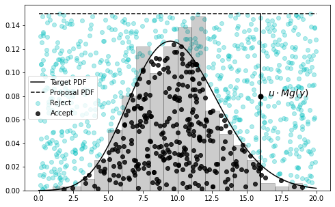
A common word-picture for this process, is to imagine a rectangular board, with the target distribution \(f(x)\) drawn across the middle. We throw darts at this board, uniformly at random, and measure the distribution of darts that fall below the \(f(x)\) line – this is an approximation of \(f(x)\). In this case, the straight top of the board represents a uniform distribution \(g(x)\).

For even more detail: first imagine the target distribution \(f(x)\), then imagine the proposal distribution \(g(x)\), scaled by a constant \(M\) to ensure it’s floating completely above \(f(x)\). Now sample a \(y\) from \(g(x)\), which gives you a coordinate along the support (the \(x\)-axis). We don’t want to keep all \(y\)’s though, we want to keep them in proportion to the probability of them being a sample of \(f\) at \(y\). So imagine picking a spot uniformly at random along the vertical line between the \(y\) on the \(x\)-axis and \(g(y)\) – we can do this by sampling \(u\sim \text{Unif}(0,1)\) and scaling by \(Mg(y)\). If the spot falls below \(f(y)\), we keep it. If not, we reject it.

Here’s a little exploration of this idea in code, with the Poisson as our target distribution, and using a uniform proposal distribution:

# bit of overkill but this package gives us flexibility
# when defining our target/proposal distributions
from functools import partial

def poisson_pmf(x, shape=1):
    return (np.power(shape, x) / factorial(x)) * np.exp(-shape)

def uniform(x, xmin=0, xmax=1):
    # little hacky but returns constant same shape as x
    return x * 0 + 1/(xmax-xmin)

xmin = 0
xmax = 20
shape = 10

# target distribution (PDF) -- let's use Poisson
f = partial(poisson_pmf, shape=shape)

# proposal distribution (PDF) -- let's use uniform
g = partial(uniform, xmin=xmin, xmax=xmax)
gsampler = np.random.uniform
M = 3  # we can be more precise here

accept = []  # list of accepted points
reject = []  # list of rejected points
for _ in range(1000):
    # get random sample from proposal distribution
    xt = gsampler(xmin, xmax)

    # now sample randomly along interval [0, Mg(y)]
    u = np.random.uniform(0,1)
    yt = u * M * g(xt) 
    if yt <= f(xt):
        accept.append([xt, yt])
    else:
        reject.append([xt, yt])
accept = np.array(accept)
reject = np.array(reject)

# compute actual, exact PDFs
xs = np.linspace(xmin, xmax, 100)
ys = f(xs)
gs = g(xs)

fig, ax = plt.subplots(1,1, figsize=(8,5))

# plot sampled histogram of target PDF
ax.hist(accept[:,0], bins=20, range=(0,20), density=True,
        color='k', edgecolor='k', alpha=0.2)

# plot scatters of accepted/rejected samples from proposal
ax.scatter(reject[:,0], reject[:,1], marker='o', c='c', alpha=0.3, label='Reject')
ax.scatter(accept[:,0], accept[:,1], marker='o', c='k', alpha=0.8, label='Accept')

# plot actual distributions
ax.plot(xs, ys, 'k-', label='Target PDF')
ax.plot(xs, gs * M, 'k--', label='Proposal PDF')

# plot instructional elements
ax.plot([16,16], [0, 0.15], 'k-')
ax.scatter([16], [0.08], c='k', s=50)
ax.text(16.5, 0.08, r'$u\cdot Mg(y)$', fontsize=14)

ax.legend(fontsize=10)

(The visualization is above.)

You may have noticed we chose \(M\) a little carelessly, just ensuring it was big enough for the proposal distribution to cover the entire target. Ideally, we want \(M\) to be as small as possible, and/or for \(g(x)\) to be as close as possible to \(f(x)\), so we don’t waste time taking a bunch of samples that will just be rejected.

Returning to the Poisson process

Back to the Poisson process. It turns out, we can apply a type of accept-reject algorithm to the Poisson process, for a non-homogeneous rate. Given a Poisson process with rate \(\lambda (t)\), such that \(\lambda (t)\leq \lambda_{\text{max}}\) for all \(t\), you can simulate a homogeneous process as before with rate \(\lambda_{\text{max}}\), but then just keep an arrival at \(t_i\) with probability \(\lambda (t_i)/\lambda_{\text{max}}\).

This isn’t exactly the same as before, but it uses the same intuition. Here’s the original proof, on page 6 (I think it’s the original, anyway).

Example

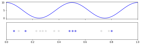
As an example, let’s say our process has some cyclical rise and fall, like rush hour, and the rate governing our process is:

(Note: we’re just using the square as a cheap way to keep the rate positive.)

Since \(\text{max} \ \cos^2(t) = 1\), our \(\lambda_{\text{max}} = 10\), which means we should observe similar behavior during peaks to our homogeneous processes previously with \(\lambda = 10\), but with very little happening elsewhere.

T = 1
maxrate = 10  

def rfun(t):
    return maxrate * (np.cos(t * (2*np.pi)) ** 2)

N_T = np.random.poisson(maxrate * T)
ts  = np.random.uniform(size=N_T)

# thinning
ts_thin = ts[np.random.uniform(size=len(ts)) <= (rfun(ts) / maxrate)].copy()

and then to visualize,

fig, axs = plt.subplots(2,1, figsize=(10,3), sharex=True)

# draw rate
xs = np.linspace(0,T,100)
axs[0].plot(xs, rfun(xs), 'b-')

# draw points
axs[1].scatter(ts, [0]*len(ts), c='k', s=50, alpha=0.1)
axs[1].scatter(ts_thin, [0]*len(ts_thin), c='b', s=50, alpha=0.4)
axs[1].set(xlim=[0, T])
axs[1].get_yaxis().set_visible(False)

Into Space

We can extend these ideas to a region \(E\in \mathbb{R}^d\) by saying the number of points \(N_B\) in any open subset \(B\subset E\) must also follow a Poisson distribution with parameter \(\lambda \vert B\vert\) where \(\vert B\vert\) represents the size (area, volume, hypervolume) of \(B\).

This is all very analogous to the 1D, temporal version, we’ve just dropped the notion of time — all the events “happen at once.” Either process above may be reinterpreted as a spatial process, if we drop the notion of time, and envision a space of dimension \(d=1\).

Spatial, with homogeneous intensity

Typically though we are modeling physical things in dimension \(d=2\) or \(d=3\). Regardless, the collection of events must still follow a Poisson, so we can follow the same approach. There’s not a way to extend the “exponential interarrival time” simulation approach to \(d\geq 2\), so we stick with using the Poisson distribution approach. Note that now, we independently distribute the samples uniformly at random both in the \(x\) and \(y\) directions.

x1, y1 = 1,1
rate = 100

# get correct number (draw from Poi(rate*area))
N_T = np.random.poisson(rate * (x1 * y1))

# get correct positions
xs = np.random.uniform(0,x1, size=N_T)
ys = np.random.uniform(0,y1, size=N_T)

and visualize,

fig, ax = plt.subplots(1,1, figsize=(8,8))
ax.scatter(xs, ys, c='b', s=50, alpha=0.3)
ax.set(xlim=[0,x1], ylim=[0,y1])

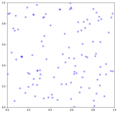
Imagine, for example, each dot is a tree in a dense forest with completely homogeneous environmental conditions.

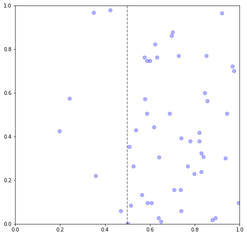
Spatial, with non-homogeneous intensity

To introduce a non-homogeneous intensity, we can mirror the same “thinning” process as before. Let’s start with a very simple example, a step function where the rate decreases sharply when \(x\) is below some threshold.

x1, y1 = 1,1

# intensity = rate if x>=5 o.w. 0
step_x = 0.5
rate = 100
def rfun(x, y):
    flag = x >= step_x
    return flag * rate + (1-flag) * (rate/10)

# get a correct number (upper bound)
N_T = np.random.poisson(rate * (x1 * y1))

# get positions
xs = np.random.uniform(0, x1, size=N_T)
ys = np.random.uniform(0, y1, size=N_T)

# thinning
# want denom to be a tight bound on rfun to get efficient thinning
ix = np.where(np.random.uniform(size=N_T) <= (rfun(xs, ys) / rate))
xs = xs[ix]
ys = ys[ix]

For one last example, let’s try something a little trickier. Let’s use a cosine function like before, but adapt to the spatial setting by having radiating ripples of high rates. Instead of parameterizing with \(x\) and \(y\), let’s use \(r\) (radius) and \(\theta\) (angle).

r = 3

def rfun(r):
    # max=2
    return 1 + np.cos(r**2)

# note \int_0^2\pi \int_0^10 1+\cos(r^2) r dr dt = ..
A = np.pi * ((r**2) + np.sin(r**2))
maxrate = 2

# draw points dist ~ Pois
NB = np.random.poisson(A)

# create points
rs = np.random.uniform(0,r, size=NB)
ts = np.random.uniform(0,2*np.pi, size=NB)

# accept-reject
ix = np.where(np.random.uniform(0,1,size=NB) <= (rfun(rs) / maxrate))[0]
rs_thin = rs[ix].copy()
ts_thin = ts[ix].copy()

Note we’re keeping track of accepted (rs_thin, ts_thin) samples separately for visualization purposes. Need to be careful with the transformations in this viz, little bit of trig:

# prep data to draw the rate function
Xm, Ym = np.meshgrid(np.linspace(-r, r, 200), np.linspace(-r, r, 200))
XX = np.array([Xm.ravel(), Ym.ravel()]).T
Z = rfun(np.sqrt(XX[:,0]**2 + XX[:,1]**2))
Z = Z.reshape(Xm.shape)

fig, ax = plt.subplots(1,1, figsize=(10,8))

# draw the rate function
cb = ax.contourf(Xm, Ym, Z, 
                 cmap='Blues', vmin=0, vmax=2,
                 alpha=0.3)

# draw the samples
ax.scatter(rs * np.cos(ts), rs * np.sin(ts), c='k', s=80, alpha=0.1)
ax.scatter(rs_thin * np.cos(ts_thin), rs_thin * np.sin(ts_thin), c='k', s=80, alpha=0.8)

# colorbar to help interpret the rate function
plt.colorbar(cb)

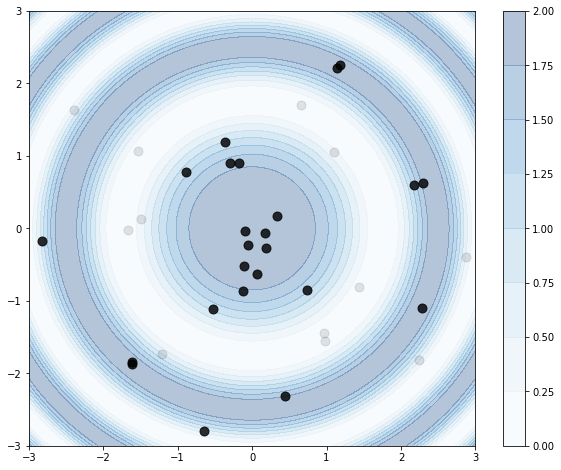
Et voilà. We see the thinning process tends to keep samples in the peaks of the rate function, as intended.

Next steps

As you’ve seen, we’ve taken a simple process – the Poisson process – and expanded its complexity and modeling power by modifying different underlying assumptions. Homogeneity, dimension, etc.

Another common way to extend this process is by making the intensity a stochastic process itself. That is, the intensity varies randomly, in a well-defined way. This creates a doubly stochastic process, also called a Cox process (after the British statistician). A common choice for the intensity is a Gaussian process, or more specifically, a log-Gaussian process (to ensure the intensity remains positive), yielding the log-Gaussian Cox process (LGCP). Again we may extend this to either temporal or spatial applications.

Another direction we may take is to break the independence assumption between events. In real applications, often the occurrence of an event increases the probability of immediate future events. One way to capture this is by defining the intensity in terms of the history of past events. The Hawkes process, for example, defines the intensity as a sum over exponentially decreasing contributions from every prior event, plus some base rate. We call this a self-exciting process, and it seems to match the bursts of events we see empirically in many applications from human interaction to earthquakes to neurons firing in the brain. (I’ve done a decent bit with this process – check out my blog about it or this Github repo with some intro-friendly Python code.)

Thanks for reading!