Autocorrelation in Elo ratings

In a previous post, I gave an interpretation of Elo ratings as weights of a logistic regression, updated online à la stochastic gradient descent.

Something that didn’t quite fit within this scheme, though, was FiveThirtyEight’s autocorrelation adjustment. I (try to) work through that why that term is what it is in this post.

Caveat. There are still several things about this that I don’t think are right: this is a working post, and I’m hoping to get some inspiration/feedback from someone out there smarter than me. :)

Motivation

FiveThirtyEight uses the following formula for their NFL Elo ratings:

where \(z\) is the game’s margin of victory, \(x=R_i^k - R_j^k\), and

Let’s just ignore ties.

My question is the specific justification for the \(A(x)\) term:

• why this form, and
• why those numbers.

I’m looking for more than a layman’s explanation, which 538 already offers and is the typical answer elsewhere. (Although this post goes a bit deeper.)

Quick intuition

So first you should buy off on the idea that given Team \(i\)’s current rating is \(R_i\), we should expect its rating after the current game to still be \(R_i\). For example, we shouldn’t ever expect Team \(i\)’s rating to increase, because if we did, “we should have rated them higher to begin with”!

Put in statistical language, this is the statement that we want \(\mathbb{E}[R_i^{k+1}\vert\text{all prev ratings}] = R_i^k\), but more on that in a second.

The typical explanation

So \(A(x)\), which again is

is intended to correct for over- or under-inflation of ratings in the model. We see the function is designed so that

• If Team \(i\) is the favorite (\(x>0\)), a loss is upweighted (\(A(x)>0\)) and a win is downweighted (\(A(x)<0\)).
• If Team \(i\) is the underdog (\(x<0\)), the opposite.

So this seems like it would correct for over-inflation of rating due to a heavy favorite, and vice-versa for a big underdog.

However, we are left with the questions: why achieve it in this way? And why use the denominator \(d=2200\)?

Gettin stats-y

We may interpret Elo ratings as a time series where each new rating depends only on the previous rating, plus some “noise.” More specifically, under this interpretation Elo assumes each team has some true rating, its mean, about which it is constantly fluctuating. This is called an autoregressive model, in our case AR(1). We are also assuming the team’s ratings are stationary, meaning (loosely) the mean stays the same over time.

(By the way, this is a different interpretation than the connection to SGD I wrote about before, but SGD and AR(1) are, in some sense, the same thing.)

Skipping some details, (I think) this all amounts to needing the next observation in the time series to, in expectation, equal our current observation. That is, \(\mathbb{E}[R_i^{k+1}\vert\text{prev ratings}] = R_i^k\).

The fact that we’re fretting about a correction term at all arises because of the margin-of-victory \(M(z)\) term we are including. This isn’t part of the “classical” Elo rating scheme, and it’s messing everything up! Without it, we have

which is just fine.

Now, including a margin-of-victory term \(M(z)\), we need

which, computing expectation over all possible game outcomes as encoded in \(z\), given \(R_i^k\) and \(R_j^k\), implies

over some distribution for the margin \(z\). Rearranging, we get

and we want some \(A(x)\) so this holds for any Elo delta \(x\).

We should be able to interpolate some function for the expected \(M(z)\)’s, and then if we are satisfied with our functional form for \(A(x)\), solve for the denominator \(d\).

Let’s try it.

In search of d

We need to (1) work out the empirical conditional expectations for \(M(z)\), then (2) approximate them with functions, and finally (3) solve for \(d\) in terms of those functions.

We can easily* pull boxscores, Elo ratings, and plot the mean \(M(z)\)’s. (*really not that easy, but see code at the bottom of this post.)

Here’s the expected \(M(z)\) given various Elo rating deltas, based on the past 18 NFL seasons.

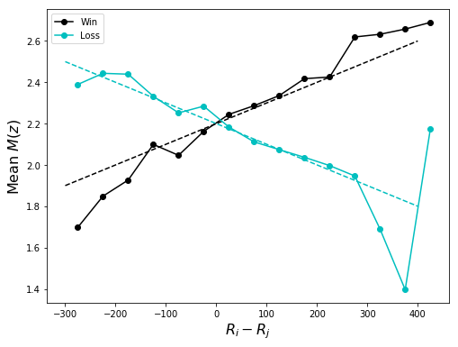
Nice! So the empirical (conditional) expectations we’re after are both reasonably approximated by linear functions:

(Let the reader note: the slope and intercept here are what you might call “eyeball” estimates, although they are quite close to an OLS estimate.)

Returning to Eq. \eqref{eq:goal} and using our satisfying functional form for \(A(x)\) from Eq. \eqref{eq:autocorr}, we (almost) have

which gives \(d=2200\). Voila!

To do. To get here, we had to ignore the \(\sigma/(1-\sigma)=10^{x/400}\) term in Eq. \eqref{eq:goal}. There might be a way to rewrite the expected \(M(z)\)’s in a way they still fit the data and cancel this other term out, but if not, I’m not sure.

Code

Fortunately we can make heavy use of 538’s public NFL data.

First some imports to get us running in a Jupyter notebook:

%matplotlib inline
import matplotlib.pyplot as plt
import pandas as pd
import numpy as np

Then we load the data, extract just the last few seasons, and run the desired stats:

box = pd.read_csv('https://raw.githubusercontent.com/fivethirtyeight/nfl-elo-game/master/data/nfl_games.csv')

# convert date to datetime
box['date'] = pd.to_datetime(box['date'])

# grab since ____ season
box = (box[box['date'] > '2003-08-01']
       .reset_index()
       .drop(['index'], axis=1)
       .copy())

n = box.shape[0]
elodiffs = np.zeros(n)
pdiffs   = np.zeros(n)
for i, row in box.iterrows():
    elodiffs[i] = row['elo1'] - row['elo2'] + (0 if row['neutral']==1 else 65)
    pdiffs[i]   = row['score1'] - row['score2']

We could do something like a pdiffs vs. elodiffs plot with Seaborn at this point, perhaps a jointplot like this …

import seaborn as sns
sns.jointplot(elodiffs / 25, pdiffs, ylim=(-50,50), kind='hex')

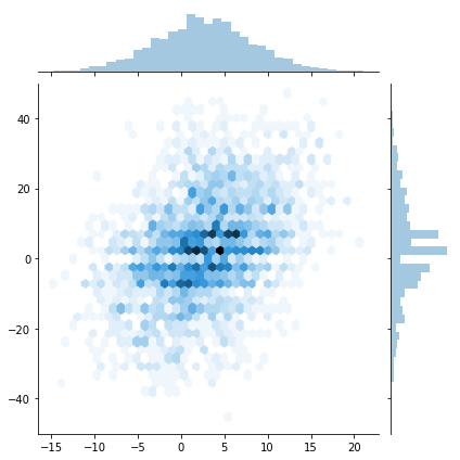
which is quite exciting. But what we’re really interested in is the mean MOV function distributions, which is the much less pretty:

xs = np.linspace(-300,400,10)

def g1(x):
    return x/1000) + 2.2
def g2(x):
    return -x/1000 + 2.2

fig, ax = plt.subplots(1,1, figsize=(8,6))

ax.plot(ed, mw, 'ko-', label='Win')
ax.plot(xs, g1(xs), 'k--')

ax.plot(ed, ml, 'co-', label='Loss')
ax.plot(xs, g2(xs), 'c--')

ax.set_xlabel(r'$R_i - R_j$', fontsize=16)
ax.set_ylabel(r'Mean $M(z)$', fontsize=16)
ax.legend()

plt.show()