Simulating a Log-Gaussian Cox Process

In a previous post, we discussed the Poisson process, and tinkered with the idea of the intensity varying over time.

Now let’s consider the idea of having the intensity itself be a stochastic process. That is, we don’t directly control the intensity, it is a random process itself. This allows us to model situations where we have random activity generated from endogeneous (“from within”) structure determined by random activity generated from exogeneous (“from without”) structure.

This setup gives us a doubly-stochastic process, or Cox process, named after the statistician David Cox who invented them. (Although some argue that an English/French guy named Maurice Quenouille invented them first.)

A lot of the material on these jumps right into the deep end with Ito calculus and measure theory. Let’s see if we can get a feel for Cox processes with some tinkering. We’ll start with the Log-Gaussian Cox Process family. (And yes, I know there are libraries out there for Python and R and others for some of these topics, but isn’t it more enlightening to make your own??)

Log-Gaussian Cox Process (LGCP)

A log-Gaussian Cox process (LGCP) is a stochastic process where the logarithm of the intensity is a Gaussian process.

Let’s unpack that a bit. We’ll start with a 1-d input space \(\mathbb{R}\) and define a Poisson process where the number of events \(N\) in an interval of length \(L\) is distributed as

where \(\Lambda = \lambda(t) L\). To make this a Cox process (and not simply a non-homogeneous Poisson process), we’ll define the intensity \(\lambda(t)\) itself as a sample from a distribution.

I assume you’re familiar with GPs, so let’s try those. If you’re not, check out this post and play around with this visualization. In brief, imagine being able to define a distribution over functions \(f \ : \ \mathbb{R}^d\rightarrow\mathbb{R}\), so you could sample one or multiple functions with similar properties (making it a process). (To get any more detailed, I recommend just reading the post.)

So for our intensity function we’ll use a function sampled from a GP. Note that a function sampled from a GP may be negative, but the intensity needs to be positive. One way to fix this, is to apply the exponential to the GP. (Or in other words, the log of the intensity gives a GP: log-Gaussian. Yea, I know, it feels backward to me too.)

We’ve now fully defined a LGCP.

Now, to simulate events from this Cox process, we can apply a thinning process as before in the simpler non-homogeneous case. We just need a rate \(\tilde{\lambda}\) (although not necessarily constant) that provides an envelope to \(\lambda(t)\) (i.e. \(\tilde{\lambda}\geq \lambda(t)\) for all \(t\)), then sample from the point process using that rate, then accept events with probability \(\lambda(t)/\tilde{\lambda}\).

import matplotlib.pyplot as plt
import numpy as np
import scipy.stats
from scipy.spatial import distance_matrix

We’ll use a “radial-basis function” kernel for our toy example. Note we have to do a few numpy maneuvers to force lists into a strict 1-d shape — there may be a slicker way around this. Otherwise, it’s a straightforward implementation of the following function:

# scipy's distance_matrix can handle different size matrices
# X -> (m,k), X_ -> (n,k), returns -> (m,n)
def rbf(X, X_, ls=1):
    # this reshapes if X or X_ are lists (1d)
    X = X.reshape((-1,1)) if len(X.shape) == 1 else X
    X_ = X_.reshape((-1,1)) if len(X_.shape) == 1 else X_

    # compute rbf and return
    return np.exp(-(1/(2*ls)) * np.power(distance_matrix(X, X_), 2))

Notice we’ll need the exact rate \(\lambda(t_i)\) for a given event \(t_i\), to determine if it is accepted or rejected by thinning. This means, we either need to include each \(t_i\) as an input to the GP, or do some sort of binning/gridding approximation. In the code below, we take the binning route (note use of numpy.searchsorted). This also allows us to compute the GP first, find its max, and use that as \(M\).

def gpcox(horizon=1, ls=0.01, n=50):
    # sample from the GP (with `n` inputs)
    xs_ = np.linspace(0,horizon,n)
    K_ = rbf(xs_, xs_, ls=ls)
    fs_ = np.random.multivariate_normal(np.zeros(n), K_)
    fs_ = np.exp(fs_)  # take exp to ensure positive
    
    # create candidate times
    M = np.amax(fs_)
    N_T = np.random.poisson(M * horizon)
    ts_ = np.sort(np.random.uniform(0,horizon, size=N_T))
    
    # thin
    rates = fs_[(np.searchsorted(fs_, ts_) - 1)] # gets fs value closest to ts
    ts_thin_ = ts_[np.random.uniform(0,1,size=len(ts_)) <= (rates / M)].copy()

    return ts_, ts_thin_, fs_, xs_

fig, axs = plt.subplots(3,1, figsize=(12,8), sharex=True, gridspec_kw={'height_ratios': [2,2,1]})

ls = 0.3
ts, ts_thin, fs, xs = gpcox(horizon=10, ls=ls, n=100)

axs[0].plot(xs, np.log(fs), 'k-')
K = rbf(xs, xs, ls=ls)
for _ in range(10):
    rfs = np.random.multivariate_normal(np.zeros(len(xs)), K)
    axs[0].plot(xs, rfs, 'k-', alpha=0.2)
axs[0].set(ylabel='$f$')

axs[1].plot(xs, fs, 'k-')
axs[1].set(ylabel=r'$exp(f)$')

axs[2].scatter(ts, [0]*len(ts), c='k', s=50, alpha=0.02)
axs[2].scatter(ts_thin, [0]*len(ts_thin), c='b', s=50, alpha=0.5)
axs[2].get_yaxis().set_visible(False)

plt.show()

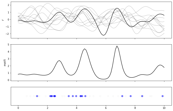
The first plot shows several samples from the GP, and highlights in black the sample chosen. The second plot shows the intensity, which is just the function sampled from the GP, with an exponential applied to it. The last plot shows a possible sequence of events resulting from this intensity – note the “rejected” events are depicted in light gray, and the “accepted” events in blue. This seems to behave as expected, with a steady stream of un-thinned events, with post-thinning events focused on areas of high intensity.

Spatial LGCP

We can extend this from \(x\in\mathbb{R}\) to \(x\in\mathbb{R}^2\) quite naturally, although the code is more involved.

# params
x1, y1 = 10, 10
m  = 30  # number partitions in grid
ls = 2   # length scale of GP

# create grid coords
xg, yg = np.linspace(0, x1, m), np.linspace(0, y1, m)
Xm, Ym = np.meshgrid(xg, yg)
X = np.array([Xm.ravel(), Ym.ravel()]).T
X += (x1 / m) / 2   # centered on grid square

# draw sample from GP
K = rbf(X, X)
Y = np.random.multivariate_normal(np.zeros(len(X)), K)

# convert to rates
Z = np.exp(Y)
zmax = np.amax(Z)

# draw Poisson
N = np.random.poisson(zmax * (x1 * y1))  
xs = np.random.uniform(0,x1, size=N)
ys = np.random.uniform(0,y1, size=N)

# now for each event (xk, yk), need to find its grid square,
# the rate there z_ij, and accept w.p. z_ij / zmax

# finds right->left (-1) index where xs occurs in xg
ix = np.searchsorted(xg, xs) - 1
iy = np.searchsorted(yg, ys) - 1

# get indices w.p. z_ij/zmax
# recall Z is (m^2), so squareform is (m,m)
# `mi` shape=N has (flat) indices in Z corresponding to grid inds from ix
# (iy,ix) because y's go down rows, x's go across columns in grid
mi = np.ravel_multi_index((iy, ix), (m,m))
kp = np.where(np.random.uniform(size=N) <= (Z[mi] / zmax))[0]

kxs = xs[kp]
kys = ys[kp]

fig, ax = plt.subplots(1,1, figsize=(10,10))

ax.contourf(Xm, Ym, Z.reshape(m,m), 
            cmap='Blues',
            levels=np.linspace(0,zmax,20))

ax.scatter(kxs, kys, c='k', s=50, alpha=0.8, zorder=1)

ax.set(xlim=[0,x1], ylim=[0,y1])
ax.set_xticks(xg, minor=True)
ax.set_yticks(yg, minor=True)
ax.grid(which='minor', color='w', linestyle='-', linewidth=0.5, alpha=0.7)
ax.tick_params(which='minor', left=False, bottom=False)  # turns off minor ticks

plt.show()

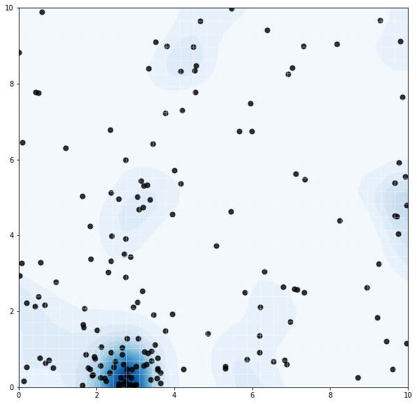
Again, we note a reasonable result of higher concentration of events in areas of high intensity. We might imagine the GP modeling nutrient concentrations, and the Poisson process modeling resulting tree growth. Or something.

Next steps

A thorough reference for LGCPs is this review by Moller, Syversveen, and Waagepetersen. They also discuss a direction we have not explored, inference of the intensity surface from data.

Other common Cox processes are Neysome-Scott cluster process and Matern cluster process (which more directly model the clustering we see in the 2-d LGCP), Thomas process, the Cox-Poisson line-point process, and others. A nice overview here.

There are also other ways to introduce additional randomness to a Poisson process via the intensity. The Cox process has the intensity process be an exogenous random process itself. The Hawkes process defines the intensity as a function of the Poisson process’s history itself (an endogenous setup) – this results in a “self-exciting” process, where arrivals increase the likelihood of future arrivals. Here’s a basic intro to this flexible model.

Thanks for reading!